This blog is written for junior PhD students to pass along the fantastic mentorship I received from my advisor and mentors during my PhD study at the University of Michigan. I’ll share tips and strategies that smoothed my PhD path, hoping they’ll illuminate yours.
Table of Contents
Coding
- Submit jobs on server and run job in parallel
- Good reference: https://sph.umich.edu/biostat/computing-old/cluster/slurm.html
- Try not to occupy all nodes at the same time
- submit jobs and leave several nodes for other people: sbatch –exclude=mulan-mc[1-6] myScript.sh
- example myScript.sh:
#!/bin/bash
#SBATCH --job-name=Yourjob  # give your job a name
#SBATCH --array=1-100%50    # this is to run 50 jobs at a time
#SBATCH --cpus-per-task=1
#SBATCH --time=24:00:00
#SBATCH --output=/net/mulan/xxx/out/Yourjob%a.txt  # you need to create the folder "/net/mulan/xxx/out"
#SBATCH --error=/net/mulan/xxx/err/Yourjob%a.txt   # same as above
#SBATCH --mem-per-cpu=5000MB
#SBATCH --partition=mulan,main                           # or just one of these partitions

bash
let k=0

for ((arg1=1;arg1<=10;arg1++)); do
	for ((arg2=1;arg2<=10;arg2++)); do
	  let k=${k}+1
	  if [ ${k} -eq ${SLURM_ARRAY_TASK_ID} ]; then
		  Rscript --verbose ./Yourcode.R   ${arg1}  ${arg2}
	  fi
	done
done
# example R script “Yourcode.R”:
args <- as.numeric(commandArgs(TRUE))
i = args[1] # simulation scenario, i.e. if you have 10 scenarios, here you are running the i-th scenario
j = args[2] # repeat number, i.e. when you need to run 10 replicates in each scenario
print("scenario")
print(i)
print("repeat")
print(j)
# then you can write your codes from here.
- Additionally, for each project, I found it beneficial to organize by creating folders within each project folder. These folders were named ‘code’, ‘result’, ‘err’, ‘out’, ‘data’, and ‘figure’.
- It is also helpful to collect and write functions to create your own “code library”, and save them into “utilities_function.R” or “utilities_function.py”, so that you can directly source them whenever needed.
- RcppArmadillo (write codes in Rcpp and then you can source the functions in R, this can help make the codes faster)
- Conda environment on server (especially useful for python packages)
- Here is the tutorial to install it: https://www.digitalocean.com/community/tutorials/how-to-install-anaconda-on-ubuntu-18-04-quickstart
- File transfer tools (between the server and your computer)
- PuTTY (file transfer client for for windows)
- Transmit (file transfer client for macOS)
- Fetch (free with educational email)
- Making figures (journals usually require 300 ppi resolution)
- In R: ggplot
- ggplot2 tutorial: https://www.cedricscherer.com/2019/08/05/a-ggplot2-tutorial-for-beautiful-plotting-in-r/
- or try some codes I summarized: https://lulushang.org/blog/Figures
- Adobe Illustrator (free with umich email. When you make figures with ggplot in R, save as pdf and then drag it into Adobe Illustrator, then you can easily edit the figure legends or colors.)
- Useful tutorial video: https://www.youtube.com/watch?v=Ib8UBwu3yGA
- Powerpoints/Keynotes
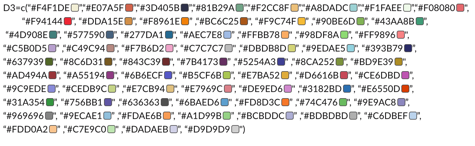
- Useful color palettes: https://coolors.co/palettes/trending
- In R: ggplot
Reading
- Reading papers
- Google scholar (follow individual researchers and subscribe through email)
- Researcher (iphone/ipad APP, receive journal updates)
- Journal websites (i.e. https://www.nature.com/nature/research-articles)
- biorxiv and arxiv
- Twitter (need to train it a little bit so that it can recommend related papers for you)
- Taking notes
- Notion (very flexible, discount with umich email)
- Evernote
Writing
- Keep track of references: EndNote, Mendeley, or Zotero
- Books: The Elements of Style; On Writing Well, …
- “Ten simple rules for structuring papers”: https://journals.plos.org/ploscompbiol/article?id=10.1371/journal.pcbi.1005619
Meeting
- These are just things that might be helpful, different people may have different styles when meeting with their advisors
- Before the weekly meeting:
- summarize the topics you want to discuss, list them from most to least important
- prepare slides or notes, organize the results and put one sentence summary on each page
- think about what questions you have, google or do as much preliminary exploration as you can
- think about possible solutions when you meet challenges, for example, when you have two options and both are easy to try, try them first and summarize the results, and then discuss the results with your advisor on the meeting. Otherwise, if both options are time consuming, you may want to ask your advisor to help rank the priority
- During the meeting:
- take notes of the topics you should follow up on, and their priority
- be honest and tell your advisor if you are stuck somewhere
- After the meeting:
- summarize what was discussed and your next steps
- send an email if you need further input from your advisor, outline what was discussed and what you need
- Other tips:
- summarize your past experience to identify what worked well and why
- this is your PhD, don’t totally rely on your advisor, you are the one to solve the problems and make things work
- Before the weekly meeting:
General stuff
- Creating your personal website
- github (i.e. https://pages.github.com); google sites; or other tools.
- analyze your website traffic: https://analytics.google.com
- Graduate study advice
- “Twenty things I wish I’d known when I started my PhD”: https://www.nature.com/articles/d41586-018-07332-x
- Tips to Become a Better Ph.D. Student: https://www.cs.princeton.edu/~ziyangx/graduate-advice/
- “The Professor is in” guidance for PhD: https://theprofessorisin.com/pearlsofwisdom/
- Matt Might’s tips for grad students: https://matt.might.net/articles/grad-student-resolutions/
- Hanna M. Wallach’s How to Be a Successful PhD Student: https://people.cs.umass.edu/~wallach/how_to_be_a_successful_phd_student.pdf
- Eric Gilbert’s guide for phd students: https://docs.google.com/document/d/11D3kHElzS2HQxTwPqcaTnU5HCJ8WGE5brTXI4KLf4dM/edit#
- Tips for PhD study: https://github.com/jbhuang0604/awesome-tips