Table of Contents
- some colors
- some packages
- increase point size in legends
- violin plot
- Venn plot
- Volcano plot
- histogram
- density plot
- barplot
- error bar plot
- pie plot
- scatter plot
- line plot
- voronoi plot
- heatmap
- heatmap change margin size and color
- QQ plot
- QQplot multiple groups
- categorical value visualization on 2d
- continuous value visualization on 2d
- calculate Moran I
- string split code
- testEnrichment
- gprofiler2, GSEA
- tryCatch skip errors
- ZIP and unzip
- read in h5ad file
- plot 2d values with clusters
some colors
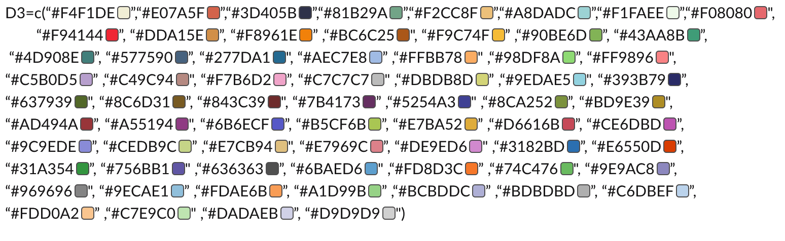
D3=c("#f4f1de","#e07a5f","#3d405b","#81b29a","#f2cc8f","#a8dadc","#f1faee","#f08080",
"#F94144", "#dda15e", "#F8961E" ,"#bc6c25", "#F9C74F" ,"#90BE6D", "#43AA8B",
 "#4D908E", "#577590", "#277DA1", "#AEC7E8" ,"#FFBB78" ,"#98DF8A", "#FF9896",
"#C5B0D5" ,"#C49C94", "#F7B6D2", "#C7C7C7" ,"#DBDB8D" ,"#9EDAE5", "#393B79",
"#637939", "#8C6D31", "#843C39", "#7B4173" ,"#5254A3" ,"#8CA252", "#BD9E39",
"#AD494A", "#A55194", "#6B6ECF", "#B5CF6B", "#E7BA52" ,"#D6616B", "#CE6DBD",
"#9C9EDE", "#CEDB9C" ,"#E7CB94", "#E7969C", "#DE9ED6" ,"#3182BD", "#E6550D",
"#31A354", "#756BB1" ,"#636363", "#6BAED6" ,"#FD8D3C" ,"#74C476", "#9E9AC8",
"#969696", "#9ECAE1" ,"#FDAE6B", "#A1D99B" ,"#BCBDDC" ,"#BDBDBD", "#C6DBEF",
"#FDD0A2" ,"#C7E9C0" ,"#DADAEB", "#D9D9D9")
some packages
library(ggplot2)
library(ggpubr)


library(reticulate)
use_python("/net/mulan/home/shanglu/anaconda3/envs/SVGPVAE/bin/python", required=TRUE)
sc <- import("scanpy")

suppressMessages(require(SPARK))
library(Seurat)
library(peakRAM)
library(ggplot2)
library(ggpubr)
library(mclust) # ARI
library(aricode)# NMI
library(SpatialPCA)# NMI
library(lisi) # lisi score
library(reticulate)
library(tidyverse)
increase point size in legends
+ guides(colour = guide_legend(override.aes = list(size=10)))
violin plot
dp <- ggplot(dat, aes(x=num, y=pve)) +
  geom_violin(trim=FALSE)+
  geom_boxplot(width=0.1, fill="white")+
  labs(title="xxx",x="xxx", y = "xxx")+
  scale_fill_brewer(palette="RdBu") +
  theme_minimal(base_size = 22)
dp
boxplot
# example 1
p <- ggplot(dat, aes(x = num, y = pve )) +
        geom_boxplot(alpha = 0.8,fill = "cornflowerblue") +
        scale_fill_manual(values=c("chocolate1","seagreen3"))+
        scale_y_continuous(name = "xxx",
                           #breaks = seq(0, 9, 1),
                           limits=c(0, 1)) +
        scale_x_discrete(name = "xxx") +
        ggtitle("xxx") +
        theme_minimal() +
        theme(plot.title = element_text(size = 18),
              text = element_text(size = 18),
              #axis.title = element_text(face="bold"),
              axis.text.x=element_text(size = 18) ,
              legend.position = "bottom")# +
        #facet_grid(. ~ Method)
p


# example 2

dat = data.frame(Method, ranking, Tissue, Tissue_types)

p10 <- ggplot(dat, aes(x = Tissue_types, y = ranking, fill = Tissue_types)) +
        geom_boxplot(alpha = 0.7) +scale_fill_manual(values=c("skyblue2","seagreen3"))+
        scale_y_continuous(name = "xxx",
                           breaks = seq(0, 40, 5),
                           limits=c(0, 40)) +
        scale_x_discrete(name = " ") +
        ggtitle(paste0(disease_name[i])) +
        theme_bw() +
        theme(plot.title = element_text(size = 20,  face = "bold"),
              text = element_text(size = 20),
              axis.title = element_text(face="bold"),
              axis.text.x=element_text(size = 15) ,
              legend.position = "bottom") +
        facet_grid(. ~ Method)
p10


# example 3

# order_dat$method_ratio = factor(order_datface$method_ratio, levels=rev(taba$method_ratio),order=T)
p2=ggplot(order_dat, aes(x=method_ratio, y=order)) +
  #geom_boxplot(alpha = 0.6,fill = "lightgreen")+
  geom_boxplot(alpha = 0.6,fill = cbp[1:7])+
  #stat_summary(fun=mean, geom="point", shape=20, size=10, color="red", fill="red") +
  # geom_abline(intercept = coefs[1], slope = coefs[2],color="orange",size=2)+
  #geom_point(shape=19, fill="#56B4E9", color="#56B4E9", size=3)+
  #geom_hline(yintercept=median(SpatialPCA_ratio), linetype="dashed", color = "red",size=1)+
  #geom_jitter(position = position_jitter(w = 0.1, h = 0),fill="#D55E00",color="#D55E00", size=1)+
  theme_bw(base_size=20)+
  #ylim(0,1)+
  #theme(axis.text.x = element_text(angle = 60,  hjust=1))+
  labs(title=paste0(""),
       x="", y = "Rank order")+
  coord_flip()
print(p2)
Venn plot
library(Vennerable)

Vcommon <- Venn(list("ePeak Genes"= ePeaks$GENE,"eGenes"= eGenes$Gene ) )
plot(Vcommon,doWeights=TRUE)


make_venn = function(plist , namelist, title){
  library(VennDiagram)
  library(RColorBrewer)
  myCol <- brewer.pal(length(plist), "Pastel2")

  venn.diagram(
        x = plist,
        category.names = namelist,
        filename = paste0("#",title,".png"),
        output=TRUE,
        # Output features
        imagetype="png" ,
        height = 480 ,
        width = 480 ,
        resolution = 300,
        compression = "lzw",
        # Circles
        lwd = 2,
        lty = 'blank',
        fill = myCol,
        # Numbers
        cex = .6,
        fontface = "bold",
        fontfamily = "sans",
        # Set names
        cat.cex = 0.6,
        cat.fontface = "bold",
        cat.default.pos = "outer",
        cat.pos = c(-27, 27, 135),
        cat.dist = c(0.055, 0.055, 0.085),
        cat.fontfamily = "sans",
        rotation = 1)


}
Volcano plot
VolcData <- allChr.est[,c("beta","pvalue","qvalue")]
VolcData$sig <- ifelse(paste(allChr.est$PEAK,allChr.est$SNP) %in% paste(reported_m6AQTL$PEAK,reported_m6AQTL$SNP),"FDR<0.1","Non-sig")

cbbPalette <- c("#000000", "#E69F00", "#56B4E9", "#009E73", "#F0E442", "#0072B2", "#D55E00", "#CC79A7")

ggplot(VolcData, aes(x = beta, y = -log10(pvalue)) )+ geom_point(size = 0.5, color =  "gray")+geom_point(data = VolcData[VolcData$sig == "FDR<0.1",],aes(x = beta, y = -log10(pvalue)), color = "#0072B2",size = 0.6 )+theme_bw()+theme(axis.title =  element_text(size = 20, face = "bold"),axis.text = element_text(size = 20, face = "bold", color = "black"),  axis.line = element_line(color = "black",size = 0.8), axis.ticks = element_line(color = "black",size = 0.8))+xlab("Effect sizes") + scale_x_continuous(limits = c(-2.5,2.5))
histogram
# example 1

ggplot(df, aes(x=df[,k])) +
  geom_histogram(bins = 150,color="darkblue", fill="lightblue")+
  geom_vline(aes(xintercept=median(df[,k])),linetype="dashed")+
  theme_minimal(base_size = 22)+
  geom_density(alpha=0.6)+
   labs(title=paste0(xxx),x=paste0(xxx), y = "xxx")

# example 2

cbbPalette <- c("#000000", "#E69F00", "#56B4E9", "#009E73", "#F0E442", "#0072B2", "#D55E00", "#CC79A7")

ggplot(data = reported_m6AQTL, aes(x = beta) )+
geom_histogram(col=I("black"),bins = 100)+
theme_bw()+
theme(axis.title =  element_text(size = 20, face = "bold"),
      axis.text = element_text(size = 15, face = "bold", color = "black"),
      axis.line = element_line(color = "black",size = 0.8),
      axis.ticks = element_line(color = "black",size = 0.8))+
xlab("Effect sizes")
density plot
# example 1

  ggplot(eqtl_table_EU2, aes(x = eqtl_table_EU_rs_dist_tss)) +
  geom_density(aes(fill = eQTL_order), alpha = 0.4) +
  geom_vline(data = mu, aes(xintercept = grp.median, color = eQTL_order), linetype = "dashed") +
  labs(title="xxx",x ="xxx")

# example 2

p1 <-
        ggplot(ct1, aes(x=pos, group=Feature,colour=factor(Feature), weight=3*weight))  +
        ggtitle("Distribution on mRNA") +
        theme(axis.ticks = element_blank(), axis.text.x = element_blank()) +
        xlab("") +
        ylab("Frequency") +
        geom_density(adjust=adjust,aes(fill=factor(Feature)),alpha=0.2,position="fill") +
        annotate("text", x = 0.5, y = -0.2, label = "5'UTR") +
        annotate("text", x = 1.5, y = -0.2, label = "CDS") +
        annotate("text", x = 2.5, y = -0.2, label = "3'UTR") +
        theme_bw() + theme(axis.ticks = element_blank(), axis.text.x = element_blank(),panel.border = element_blank(), panel.grid.major = element_blank(),
                           panel.grid.minor = element_blank(), axis.line = element_line(colour = "black")) +
        annotate("rect", xmin = 0, xmax = 1, ymin = -0.12, ymax = -0.08, alpha = .99, colour = "black")+
        annotate("rect", xmin = 2, xmax = 3, ymin = -0.12, ymax = -0.08, alpha = .99, colour = "black")+
        annotate("rect", xmin = 1, xmax = 2, ymin = -0.16, ymax = -0.04, alpha = .2, colour = "black")
barplot
# example 1
p1 =ggplot(dat, aes(x=methods, y=value,fill=methods)) +
	  geom_bar(stat="identity", color="black",width=0.8)+
  #scale_fill_brewer(palette="Paired")+
  #scale_fill_brewer(palette="Set3")+
  #scale_fill_distiller(palette = "Oranges")+
  scale_fill_manual(values = D3)+
  labs(title=paste0("Sample ",name[sample]))+
  theme(legend.position="right") +
  theme_classic()+
  	  #geom_abline(intercept = coefs[1], slope = coefs[2],color="orange",size=2)+
	  #geom_point(shape=19, fill="#56B4E9", color="#56B4E9", size=3)+
	  #geom_jitter(position = position_jitter(w = 0.1, h = 0),fill="#D55E00",color="#D55E00", size=1)+
	  #ylim(0,1)+
  #geom_hline(yintercept=median(dat[1,metrics+1]), linetype="dashed", color = "red",size=1)+
  #scale_fill_manual(values = method_color)+
  theme(axis.text.x = element_text(angle = 60,  hjust=1))+
  theme(plot.title = element_text(size = 30),
              text = element_text(size = 30),
              #axis.title = element_text(face="bold"),
              #axis.text.x=element_text(size = 20) ,
              legend.position = "right")+
  facet_wrap(~variable)+
  labs(title=paste0(""),
   x="Methods", y = paste0("ARI"))

# example 2
p=ggplot(data=datt, aes(x=fct_reorder(tolower(term_id),log10p), y=log10p, fill=Source,label = ifelse(significant ==TRUE, "*",""))) +
  geom_bar(stat="identity", position=position_dodge(),color="black",width=0.8)+
  #scale_fill_continuous(low='#F0E442', high='red', guide=guide_colorbar(reverse=TRUE)) +
  scale_fill_manual(values = c("#00AFBB", "#E7B800", "#FC4E07", "#56B4E9", "#009E73","#F0E442", "#0072B2", "#D55E00", "#CC79A7"))+
  labs(title=paste0("Pseudotime related genes GSEA"),x="Biological terms", y = "-log10(p value)")+
  coord_flip()+
  theme_classic()+
  #geom_text(vjust = 0.5) +
  geom_hline(yintercept=-log10(0.05), linetype="dashed", color = "red",size=2)+
  geom_text(vjust = 1, nudge_y = 0.5)+
  #ylim(0,1)+
    theme(plot.title = element_text(size = 30,color="black",face="bold"),
              text = element_text(size = 30,color="black",face="bold"),
              #axis.title = element_text(size = 25,color="black",face="bold"),
              axis.text.x=element_text(size = 30,color="black",face="bold") ,
              legend.position = "right")# +


# example 3
ggplot(data=dat, aes(x=topcount, y=count, fill=method)) +
  geom_bar(stat="identity", position=position_dodge())+
  scale_fill_brewer(palette="Paired")+
  labs(title="xxx",x="xxx", y = "xxx")+
  theme_minimal(base_size = 22)+
  theme(legend.position="bottom")
error bar plot
# reference: m6A nature genetics paper
torus.enrich <- read.table("~/m6AQTL/m6A_QTL_results/linear_model/annotation/m6AQTL.AnnotationEnrich.est", sep = "\t")[-c(1),]
torus.enrich <- gsub("\\s+", "\t", sapply(torus.enrich,trimws))
torus.enrich <- do.call(rbind.data.frame, strsplit(torus.enrich, split = "\t") )
torus.enrich[,-c(1)] <- apply(torus.enrich[,-c(1)],2, function(x) as.numeric(as.character(x)) )

colnames(torus.enrich) <- c("feature","LogOddRatio","CI05","CI95")
torus.enrich$feature <- factor( c( "5' UTR","3' UTR", "CDS", "Intron", "Intergenic\nrepressive" ))
torus.enrich$feature <- factor( c( "5' UTR","3' UTR", "CDS", "Intron" , "Intergenic\nrepressive"), levels = torus.enrich[order(torus.enrich$LogOddRatio),"feature"] )

ggplot(torus.enrich,aes(x = LogOddRatio/log(2), y = feature ))+geom_point(size = 2)+ xlab("Log2 enrichment")+
  geom_errorbarh(aes(xmin = CI05/log(2), xmax = CI95/log(2), height = 0.3),size = 0.8)+
  theme_bw()  + ylab("Features")+
  geom_vline(xintercept = 0,linetype="dotted", colour = "red")+theme(axis.ticks = element_blank(),
                     panel.grid.minor = element_blank(), axis.line = element_line(colour = "black"), axis.text = element_text(face="bold",size = 23, colour = "black"),axis.text.y = element_text(angle = 10),axis.title.x = element_text(face="bold",size = 20) , axis.title.y = element_blank())+coord_cartesian(xlim=c(-9,6))


# Use 80% confidence intervals
p <- ggplot(pi1_phenotypes.df,
            aes(x=phenotypes, y=pi1, fill=thresh_nlogP)) +
  geom_bar(position=position_dodge(), stat="identity") +
  geom_errorbar(aes(ymin=ci10, ymax=ci90),
                width=.2,                    # Width of the error bars
                position=position_dodge(.9)) +
  labs(title = "QTL sharing (ascertained on m6A-QTLs)",
       x = "\nAscertainment cutoff",
       y = expression(paste("Sharing (", pi["1"], ")")),
       fill = expression(paste(-log[10], " p-value"))) +
  coord_cartesian(ylim=c(0,0.8)) +
  scale_fill_manual(values=cbbPalette) +
  theme_minimal() +
  theme(legend.position="bottom")
pie plot
df = data.frame("State" = statenames,"Percentage" = statenum)
library(ggplot2)

pie = ggplot(df, aes(x="", y=Percentage, fill=State)) + geom_bar(stat="identity", width=1)
pie = pie + coord_polar("y", start=0) + geom_text(aes(label = paste0(round(Percentage*100), "%")), position = position_stack(vjust = 0.5))
pie = pie + scale_fill_brewer(palette = "Set3")
pie = pie + labs(x = NULL, y = NULL, fill = NULL, title = "State")
pie = pie + theme_classic() + theme(axis.line = element_blank(),
          axis.text = element_blank(),
          axis.ticks = element_blank(),
          plot.title = element_text(hjust = 0.5, color = "#666666"))
pie
scatter plot
# example 1

ggplot(mydata, aes(x=originalranking, y=subs)) +
  geom_point(shape=19, fill="#56B4E9", color="#56B4E9", size=3)+
  geom_smooth(method=lm, se=FALSE, fullrange=TRUE,color="tomato1")+
  theme_bw(base_size=25)+
  labs(title=paste0("xxx"),
       x="xxx", y = "xxx")
dev.off()

# example 2

figure =ggplot(datt, aes(x = x, y = -y, color = region)) +
        geom_point(size=pointsize[sample], alpha = 1) +
        scale_color_viridis(option=coloroption)+
        #ggtitle(paste0("sample ",name[sample],": ",regionID))+
        ggtitle(paste0(regionID))+
        theme_void()+
        theme(plot.title = element_text(size = textsize),
            text = element_text(size = textsize),
            legend.position = "bottom")

# example 3

ggplot(effectSize_melt,aes(x = m6A, y = value))+
geom_point( size = 1)+
ylab("QTL effect sizes")+
xlab("m6A effect size")+
stat_smooth(aes(x = m6A, y = value),method = 'lm')+
facet_wrap(facets = "variable", nrow = 2 ) +
  geom_hline(yintercept = 0, lty= 2,colour="#990000")+
  theme_bw() +
  theme(panel.grid = element_blank(),
        axis.line = element_line(colour = "black",size = I(0.5)),
        axis.title = element_text(family = "arial", face = "bold", size = 15),
        axis.text = element_text(family = "arial", face = "bold", size = 14,colour = "black"),
        plot.title = element_text(family = "arial", face = "bold", size = 14, hjust = 0.5),
        legend.position = "none", strip.text = element_text(face = "bold", size = 14),
        panel.grid.minor = element_blank() )+
  stat_poly_eq(aes(label = paste(..rr.label..)),
      label.x.npc = 0.33, label.y.npc = 0.9, formula = y~x, parse = TRUE, size = 4.6,coef.digits = 2) +
  xlim(-5,5) + ylim(-5,5) + ## remove outliers, abs(effect size) > 5
  coord_cartesian(xlim = c(-2.2,2.2), ylim = c(-2.2,2.2)) ## zoom in range: c(-2.2,2.2)
line plot
ggplot(topss, aes(x=tis, y=reproducibility)) +
  geom_point(shape=19, fill="hotpink1", color="hotpink1", size=3)+
  geom_line() +
  geom_smooth(method=lm, se=FALSE, fullrange=TRUE,color="tomato1")+
  theme_bw(base_size=25)+
  ylim(0,1)+
  labs(title=paste0("xxx"),
       x="xxx", y = "xxx")
dev.off()


#  y: #eQTLs, x: #PCs
PC = c(0,  5, 10, 15, 20)
nG = PC_eQTL
nPC = length(PC)
pdf("xxx.pdf", 4,3)
plot(0, 0, xlim=c(0, 20), ylim=c(0, 600000), type="n", xlab="Number of Genotype PCs", ylab="Number of eSNPs", main="",cex.lab=1.2)
abline(v=seq(0, 20, 5), lty=2, col="lightgrey")
abline(h=seq(0, 600000, 50000), lty=2, col="lightgrey")
points(PC, nG, type="o", col=COL[2], pch=20, lwd=2)
#legend("bottomright", legend=c("eQTLs vs PCs at 5% FDR in African American"), fill=c(COL[1], "grey"), bg="white", cex=1.2)
voronoi plot
library(ggforce)


dat = data.frame(data_use$location_use, "region"=SpatialPCA_region,"expression"=data_use$SCTscaled[which(rownames(data_use$SCTscaled)=="FETUB"),])

dat_random = dat[sample(1:3813,200,replace=F),]

pdf("test.pdf",width=10,height=10)
color_in = c("#e07a5f","#a8dadc","#F9C74F")
p=ggplot(dat_random, aes(x, y)) +
  geom_voronoi_tile(aes(fill = region,group = -1L), colour = 'white',
                    expand = unit(-.5, 'mm'), radius = unit(2, 'mm'))+
  # geom_voronoi_segment(aes(fill = region,group = -1L)) +
  theme_void() +
   scale_color_manual(values = color_in)+
   theme(plot.title = element_text(size = 20,  face = "bold"),
              text = element_text(size = 20),
              axis.title = element_text(),
              axis.text.x=element_text() ,
              legend.position = "right") +
    guides(colour = guide_legend(override.aes = list(size=20)))
print(p)

lowcolor="#05a8aa"
midcolor="#edede9"
highcolor="#bc412b"
dat_random$expression[which(dat_random$region !="Tumor")]=0
p=ggplot(dat_random, aes(x, y)) +
  geom_voronoi_tile(aes(fill = expression,group = -1L), colour = 'white',
                    expand = unit(-.5, 'mm'), radius = unit(2, 'mm'))+
  geom_voronoi_segment(aes(fill = region,group = -1L)) +
  scale_color_gradient2( low=lowcolor,mid=midcolor, high=highcolor)+
   theme_void() +
   theme(plot.title = element_text(size = 20,  face = "bold"),
              text = element_text(size = 20),
              axis.title = element_text(),
              axis.text.x=element_text() ,
              legend.position = "right") +
    guides(colour = guide_legend(override.aes = list(size=20)))
print(p)
dev.off()
heatmap
mapDrugToColor<-function(annotations){
    colorsVector = ifelse(annotations["category"]=="Others",
        "blue", ifelse(annotations["category"]=="Brain related",
        "green", "red"))
    return(colorsVector)
}

testHeatmap3<-function(logCPM, annotations) {
    sampleColors = mapDrugToColor(annotations)

    # Assign just column annotations
    heatmap3(logCPM, margins=c(16,16), ColSideColors=sampleColors,scale="none")
    # Assign column annotations and make a custom legend for them
    heatmap3(logCPM, margins=c(16,16), ColSideColors=sampleColors, scale="none",
        legendfun=function()showLegend(legend=c("Others",
        "Brain related", "Colon related"), col=c("blue", "green", "red"), cex=1))

    # Assign column annotations as a mini-graph instead of colors,
    # and use the built-in labeling for them
    ColSideAnn<-data.frame(Drug=annotations[["category"]])
    heatmap3(logCPM,ColSideAnn=ColSideAnn,
        ColSideFun=function(x)showAnn(x),
        ColSideWidth=0.8)
}

category = c(rep("Others",6),rep("Brain related",3),rep("Others",3),"Colon related",
"Colon related", rep("Others",16),"Colon related","Others","Colon related",rep("Others",5))

gAnnotationData = data.frame(tissue_name, category)
gLogCpmData = a

pdf("Tissue_GTEx_heatmap_unscaled.pdf",width=7, height=7)
diag(gLogCpmData)=1
testHeatmap3(gLogCpmData, gAnnotationData)
dev.off()
heatmap change margin size and color
library(BiRewire)
library(corrplot)
library(heatmap3)

#---------------------------------
# Tissues
#---------------------------------

load("tissue_net.RData")
load("tissue_name.RData")
Tissue_network = tissue_net

# calculate Jaccard Index between each pair of tissues

a = matrix(0,38,38)
for(i in 1:38){
	for(j in (i+1):38){
		a[i,j] = birewire.similarity( Tissue_network[[i]],Tissue_network[[j]])
		a[j,i] = a[i,j]
	}
	print(i)
	print(a[i,])
}
colnames(a) = tissue_name
rownames(a) = tissue_name

# use heatmap3
mapDrugToColor<-function(annotations){
    colorsVector = ifelse(annotations["category"]=="Others",
        "blue", ifelse(annotations["category"]=="Brain related",
        "green", "red"))
    return(colorsVector)
}
testHeatmap3<-function(logCPM, annotations) {
    sampleColors = mapDrugToColor(annotations)

    # Assign just column annotations
    heatmap3(logCPM, margins=c(10,10), ColSideColors=sampleColors,scale="none",col = colorRampPalette(c("firebrick", "yellow", "white"))(1024))
    # Assign column annotations and make a custom legend for them
    heatmap3(logCPM, margins=c(10,10), ColSideColors=sampleColors, scale="none",col = colorRampPalette(c("firebrick", "yellow", "white"))(1024),
        legendfun=function()showLegend(legend=c("Others",
        "Brain related", "Colon related"), col=c("blue", "green", "red"), cex=1))

    # Assign column annotations as a mini-graph instead of colors,
    # and use the built-in labeling for them
    ColSideAnn<-data.frame(Drug=annotations[["category"]])
    heatmap3(logCPM,ColSideAnn=ColSideAnn,
        ColSideFun=function(x)showAnn(x),
        margins=c(10,10),
        ColSideWidth=0.8)
}
category = c(rep("Others",6),rep("Brain related",3),rep("Others",3),"Colon related",
"Colon related", rep("Others",16),"Colon related","Others","Colon related",rep("Others",5))
gAnnotationData = data.frame(tissue_name, category)
gLogCpmData = a
pdf("Tissue_GTEx_heatmap_unscaled.pdf",width=8, height=8)
diag(gLogCpmData)=1
testHeatmap3(gLogCpmData, gAnnotationData)
dev.off()
QQ plot
https://uw-gac.github.io/topmed_workshop_2017/association-tests.html#association-testing-with-aggregate-units
library(ggplot2)
qqPlot <- function(pval) {
    pval <- pval[!is.na(pval)]
    n <- length(pval)
    x <- 1:n
    dat <- data.frame(obs=sort(pval),
                      exp=x/n,
                      upper=qbeta(0.025, x, rev(x)),
                      lower=qbeta(0.975, x, rev(x)))

    ggplot(dat, aes(-log10(exp), -log10(obs))) +
        geom_line(aes(-log10(exp), -log10(upper)), color="gray") +
        geom_line(aes(-log10(exp), -log10(lower)), color="gray") +
        geom_point() +
        geom_abline(intercept=0, slope=1, color="red") +
        xlab(expression(paste(-log[10], "(expected P)"))) +
        ylab(expression(paste(-log[10], "(observed P)"))) +
        theme_bw()
}

qqPlot(assoc$Wald.pval)
QQplot multiple groups
I modified the codes from https://genome.sph.umich.edu/wiki/Code_Sample:_Generating_QQ_Plots_in_R
so that the points won’t be along the y-axis when we observe many small p values
library(lattice)
qqunif.plot<-function(pvalues,
	should.thin=T, thin.obs.places=2, thin.exp.places=2,
	xlab=expression(paste("Expected (",-log[10], " p-value)")),
	ylab=expression(paste("Observed (",-log[10], " p-value)")),
	draw.conf=TRUE, conf.points=1000, conf.col="lightgray", conf.alpha=.05,
	already.transformed=FALSE, pch=20,
	aspect="iso",
	prepanel=prepanel.qqunif,
	par.settings=list(superpose.symbol=list(pch=pch)), ...) {


	#error checking
	if (length(pvalues)==0) stop("pvalue vector is empty, can't draw plot")
	if(!(class(pvalues)=="numeric" ||
		(class(pvalues)=="list" && all(sapply(pvalues, class)=="numeric"))))
		stop("pvalue vector is not numeric, can't draw plot")
	if (any(is.na(unlist(pvalues)))) stop("pvalue vector contains NA values, can't draw plot")
	if (already.transformed==FALSE) {
		if (any(unlist(pvalues)==0)) stop("pvalue vector contains zeros, can't draw plot")
	} else {
		if (any(unlist(pvalues)<0)) stop("-log10 pvalue vector contains negative values, can't draw plot")
	}


	grp<-NULL
	n<-1
	exp.x<-c()
	if(is.list(pvalues)) {
		nn<-sapply(pvalues, length)
		rs<-cumsum(nn)
		re<-rs-nn+1
		n<-min(nn)
		if (!is.null(names(pvalues))) {
			grp=factor(rep(names(pvalues), nn), levels=names(pvalues))
			names(pvalues)<-NULL
		} else {
			grp=factor(rep(1:length(pvalues), nn))
		}
		pvo<-pvalues
		pvalues<-numeric(sum(nn))
		exp.x<-numeric(sum(nn))
		for(i in 1:length(pvo)) {
			if (!already.transformed) {
				pvalues[rs[i]:re[i]] <- -log10(pvo[[i]])
				exp.x[rs[i]:re[i]] <- -log10((rank(pvo[[i]], ties.method="first")-.5)/nn[i])
			} else {
				pvalues[rs[i]:re[i]] <- pvo[[i]]
				exp.x[rs[i]:re[i]] <- -log10((nn[i]+1-rank(pvo[[i]], ties.method="first")-.5)/(nn[i]+1))
			}
		}
	} else {
		n <- length(pvalues)+1
		if (!already.transformed) {
			exp.x <- -log10((rank(pvalues, ties.method="first")-.5)/n)
			pvalues <- -log10(pvalues)
		} else {
			exp.x <- -log10((n-rank(pvalues, ties.method="first")-.5)/n)
		}
	}


	#this is a helper function to draw the confidence interval
	panel.qqconf<-function(n, conf.points=1000, conf.col="gray", conf.alpha=.05, ...) {
		require(grid)
		conf.points = min(conf.points, n-1);
		mpts<-matrix(nrow=conf.points*2, ncol=2)
        	for(i in seq(from=1, to=conf.points)) {
            		mpts[i,1]<- -log10((i-.5)/n)
            		mpts[i,2]<- -log10(qbeta(1-conf.alpha/2, i, n-i))
            		mpts[conf.points*2+1-i,1]<- -log10((i-.5)/n)
            		mpts[conf.points*2+1-i,2]<- -log10(qbeta(conf.alpha/2, i, n-i))
        	}
        	grid.polygon(x=mpts[,1],y=mpts[,2], gp=gpar(fill=conf.col, lty=0), default.units="native")
    	}

	#reduce number of points to plot
	if (should.thin==T) {
		if (!is.null(grp)) {
			thin <- unique(data.frame(pvalues = round(pvalues, thin.obs.places),
				exp.x = round(exp.x, thin.exp.places),
				grp=grp))
			grp = thin$grp
		} else {
			thin <- unique(data.frame(pvalues = round(pvalues, thin.obs.places),
				exp.x = round(exp.x, thin.exp.places)))
		}
		pvalues <- thin$pvalues
		exp.x <- thin$exp.x
	}
	gc()

	prepanel.qqunif= function(x,y,...) {
		A = list()
		A$xlim = range(x)*1.02
		A$xlim[1]=0
		A$ylim = range(y)*1.02
		A$ylim[1]=0
		return(A)
	}

	#draw the plot
	xyplot(pvalues~exp.x, groups=grp, xlab=xlab, ylab=ylab,
		#aspect=aspect,
		prepanel=prepanel,
		scales=list(axs="i"),
		pch=pch,
		panel = function(x, y, ...) {
			if (draw.conf) {
				panel.qqconf(n, conf.points=conf.points,
					conf.col=conf.col, conf.alpha=conf.alpha)
			};
			panel.xyplot(x,y, ...);
			panel.abline(0,1);
		}, par.settings=par.settings, ...
	)
}

my.pvalue.list<-list("AA"=mydat[mydat$Population=="AA",1], "EA"=mydat[mydat$Population=="EA",1],
"AFA"=mydat[mydat$Population=="AFA",1],"CAU"=mydat[mydat$Population=="CAU",1],
"HIS"=mydat[mydat$Population=="HIS",1])

pdf(paste0("QQ_trait",traits[traitnum],"_test.pdf") ,width = 6, height = 6)
qqunif.plot(my.pvalue.list, auto.key=list(corner=c(.95,.05)))
dev.off()
categorical value visualization on 2d
plot_cluster = function (location, clusterlabel, pointsize = 3, text_size = 15, shape=16,title_in, color_in, legend = "none"){
    cluster = clusterlabel
    loc_x = location[, 1]
    loc_y = location[, 2]
    datt = data.frame(cluster, loc_x, loc_y)
    p = ggplot(datt, aes(x = location[, 1], y = location[, 2],
        color = cluster)) + geom_point(alpha = 1, size = pointsize,shape=shape) +
        scale_color_manual(values = color_in) + ggtitle(paste0(title_in)) +
        theme_void() + theme(plot.title = element_text(size = text_size,
        face = "bold"), text = element_text(size = text_size),
        legend.position = legend)
    p
}
continuous value visualization on 2d
library(ggplot2)
# location is n by 2 matrix of location coordinates
# feature is a vector of gene expression
plot_factor_value= function(location, feature, textmethod="Your figure", pointsize = 2, textsize = 15,shape=15)
{
    location = as.data.frame(location)
        locc1 = location[, 1]
        locc2 = location[, 2]
        datt = data.frame(feature, locc1, locc2)
        p = ggplot(datt, aes(x = locc1, y = locc2, color = feature)) +
            geom_point(size = pointsize, alpha = 1,shape=shape) +
            #scale_color_viridis(option="magma")+
			      scale_color_gradient2( low="#05a8aa",mid="#edede9", high="#bc412b")+
            ggtitle(paste0(textmethod)) +
            theme_void() +
            theme(plot.title = element_text(size = textsize),
            text = element_text(size = textsize), legend.position = "right")

    return(p)
}


plot_factor_value= function (location, feature, textmethod, pointsize = 2, textsize = 15,shape=15,lowcolor="#05a8aa",midcolor="#edede9",highcolor="#bc412b")
{
    location = as.data.frame(location)
        locc1 = location[, 1]
        locc2 = location[, 2]
        datt = data.frame(feature, locc1, locc2)
        p = ggplot(datt, aes(x = locc1, y = locc2, color = feature)) +
            geom_point(size = pointsize, alpha = 1,shape=shape) +
            #scale_color_viridis(option="magma")+
      scale_color_gradient2( low=lowcolor,mid=midcolor, high=highcolor)+
            ggtitle(paste0(textmethod)) +
            theme_void() +
            theme(plot.title = element_text(size = textsize),
            text = element_text(size = textsize), legend.position = "right")

    return(p)
}


plot_factor_value_darkmode =function (location, feature, textmethod, pointsize = 2, textsize = 15,shape=15,lowcolor="#ffffff",midcolor="#118ab2",highcolor="#284b63",legend="right")
{
    location = as.data.frame(location)
        locc1 = location[, 1]
        locc2 = location[, 2]
        datt = data.frame(feature, locc1, locc2)
        p = ggplot(datt, aes(x = locc1, y = locc2, color = feature)) +
            geom_point(size = pointsize, alpha = 1,shape=shape) +
            #scale_color_viridis(option="magma")+
      scale_color_gradient2( low=lowcolor,mid=midcolor, high=highcolor)+
            ggtitle(paste0(textmethod)) +
            theme_dark() +
            #theme_void() +
            theme(axis.line=element_blank(),axis.text.x=element_blank(),
            axis.text = element_text(size = textsize),
            plot.title = element_text(size = textsize),
          axis.text.y=element_blank(),axis.ticks=element_blank(),
          axis.title.x=element_blank(),
          axis.title.y=element_blank(),
          legend.position=legend,
          #panel.background=element_blank(),
          panel.border=element_blank(),panel.grid.major=element_blank(),
          panel.grid.minor=element_blank(),plot.background=element_blank())

    return(p)
}
calculate Moran I
get_moranI = function(count_in,location){
    # count_in: gene by spot

    count_in = as.matrix(count_in)
    if(length(which(rowSums(count_in)==0))>0){
        count_in = count_in[-which(rowSums(count_in)==0),]
    }
    library(moranfast)
    output <- apply(count_in, 1, function(x) moranfast(x, location[,1], location[,2]))
    out =  sapply(output, '[[', 1)
    return(out)
}


# spatialpc_moranI = get_moranI(SpatialPCA_result$SpatialPCs[1:5,], SpatialPCA_result$location)
# pc_moranI = get_moranI(PCA_result$PCs[1:5, ], SpatialPCA_result$location)


get_moranI_normalize = function(expr,location){
    # count_in: gene by spot

    library(moranfast)
    output <- apply(expr, 1, function(x) moranfast(x, location[,1], location[,2]))
    out =  sapply(output, '[[', 1)
    return(out)
}
string split code
strsplit_func = function(input){
  strsplit(input, split = "-")[[1]][1]
}


unlist(lapply(gostres$result$term_id,strsplit_func))
testEnrichment
testEnrichment = function(Goi, gsets, background,  mindiffexp=2) {
  scores = do.call(rbind.data.frame, lapply(names(gsets), function(gsetid){
    gset = gsets[[gsetid]]

    # much faster than using table
    tp = length(intersect(Goi, gset))
    fn = length(Goi) - tp
    fp = length(gset) - tp
    tn = length(background) - tp - fp - fn

    contingency_table = matrix(c(tp, fp, fn, tn), 2, 2)

    if (contingency_table[1,1] < mindiffexp){
      return(NULL)
    }

    fisher_result = stats::fisher.test(contingency_table, alternative="two.sided",conf.int = TRUE)
    list(pval=fisher_result$p.value, odds=fisher_result$estimate, odds_conf_low = fisher_result$conf.int[1],odds_conf_high = fisher_result$conf.int[2],found=contingency_table[1,1], gsetid=gsetid)
  }))
  if (nrow(scores) > 0) {
    scores$qval = stats::p.adjust(scores$pval, method="fdr")
  }
  scores
}
gprofiler2, GSEA
library(ActivePathways)

gmt <- read.GMT("/net/mulan/disk2/shanglu/Projects/spatialPCA/manuscript_v5/h.c24557all.v7.4.symbols.filter.gmt")
gmt_filter = gmt[c(1,2)]
count = 0
for(item in 1:length(gmt)){
  itemid = gmt[[item]]$id
  if(length(grep("CANCER MODULE",itemid))!=0  | length(grep("GOBP",itemid))!=0 | length(grep("GOCC",itemid))!=0 | length(grep("GOMF",itemid))!=0){
    count = count + 1
    print(count)
    gmt_filter[[count]]=gmt[[item]]
  }
}
write.GMT(gmt_filter, "/net/mulan/disk2/shanglu/Projects/spatialPCA/manuscript_v5/h.c24557all.v7.4.symbols.filter.update.gmt")
upload_GMT_file(gmtfile = "/net/mulan/disk2/shanglu/Projects/spatialPCA/manuscript_v5/h.c24557all.v7.4.symbols.filter.update.gmt")


library(MAST)
library(fdrtool)
library(qvalue)

library(gprofiler2)
library(ggplot2)
library(tidyverse)


h: hallmark gene sets hallmark gene sets as Gene Symbols  h.all.v7.4.symbols.gmt
C1: positional gene sets Gene sets corresponding to each human chromosome and each cytogenetic band.
c2: curated gene sets KEGG gene sets as Gene Symbols  c2.cp.kegg.v7.4.symbols.gmt
C3: regulatory target gene sets Gene sets representing potential targets of regulation by transcription factors or microRNAs.
c4: computational gene sets cancer modules as Gene Symbols  c4.cm.v7.4.symbols.gmt
c5: Ontology gene sets all GO gene sets as Gene Symbols  c5.go.v7.4.symbols.gmt
c5: Ontology gene sets Human Phenotype Ontology as Gene Symbols  c5.hpo.v7.4.symbols.gmt
C6: oncogenic signature gene sets Gene sets that represent signatures of cellular pathways which are often dis-regulated in cancer.
c7: immunologic signature gene sets all immunologic signature gene sets as Gene Symbols c7.all.v7.4.symbols.gmt
C8: cell type signature gene sets Gene sets that contain curated cluster markers for cell types identified in single-cell sequencing studies of human tissue.

# GMT downloaded in : /net/mulan/disk2/shanglu/Projects/datasets/msigdbr


upload_GMT_file(gmtfile = "/net/mulan/disk2/shanglu/Projects/spatialPCA/manuscript_v5/h.c24557all.v7.4.symbols.filter.update.gmt")
# gp__WcnH_hRul_jhQ


bg = rownames(SpatialPCA_result$rawcount)
gostres <- gost(query = unlist(ST_pseudotime_genelist),
                organism = "gp__WcnH_hRul_jhQ", ordered_query = FALSE,
                multi_query = FALSE, significant = FALSE, exclude_iea = FALSE,
                measure_underrepresentation = FALSE, evcodes = FALSE,
                user_threshold = 0.05, correction_method = "g_SCS",
                domain_scope = "custom", custom_bg = bg,
                numeric_ns = "",
                #sources = c("GO:MF","GO:BP", "GO:CC","KEGG"),
                as_short_link = FALSE)
gostres$result = gostres$result[order(gostres$result$p_value),]
gostres$result$Source = unlist(lapply(gostres$result$term_id,strsplit_func))
gostres$result$Source[which(gostres$result$Source=="MODULE")]="CANCER MODULE"
datt = gostres$result[1:10,]
datt$log10p = -log10(datt$p_value)


p=ggplot(data=datt, aes(x=fct_reorder(tolower(term_id),log10p), y=log10p, fill=Source,label = ifelse(significant ==TRUE, "*",""))) +
  geom_bar(stat="identity", position=position_dodge(),color="black",width=0.8)+
  #scale_fill_continuous(low='#F0E442', high='red', guide=guide_colorbar(reverse=TRUE)) +
  scale_fill_manual(values = c("#00AFBB", "#E7B800", "#FC4E07", "#56B4E9", "#009E73","#F0E442", "#0072B2", "#D55E00", "#CC79A7"))+
  labs(title=paste0("Pseudotime related genes GSEA"),x="Biological terms", y = "-log10(p value)")+
  coord_flip()+
  theme_classic()+
  #geom_text(vjust = 0.5) +
  geom_hline(yintercept=-log10(0.05), linetype="dashed", color = "red",size=2)+
  geom_text(vjust = 1, nudge_y = 0.5)+
  #ylim(0,1)+
    theme(plot.title = element_text(size = 30,color="black",face="bold"),
              text = element_text(size = 30,color="black",face="bold"),
              #axis.title = element_text(size = 25,color="black",face="bold"),
              axis.text.x=element_text(size = 30,color="black",face="bold") ,
              legend.position = "right")# +


pdf(paste0("ST_GSEA_pseudotime_genes.pdf"),width=40,height=5)
  print(p)
dev.off()
tryCatch skip errors
tryCatch({
    celltype_in = as.matrix(celltype_proportion_in[,num_celltype])
    sparkXw <- SPARK::sparkx(count_in, location_in,X_in=celltype_in,numCores = 5,verbose=FALSE)
    dat = data.frame("gene"=rownames(sparkXw$res_mtest),"combinedPval"=sparkXw$res_mtest$combinedPval,"sparkXw_adj_p"=sparkXw$res_mtest$adjustedPval,"celltype"=colnames(celltype_proportion_in)[num_celltype])
    save(dat, file = paste0("/net/mulan/disk2/shanglu/Projects/explore/celltype_SVG/10X_visium_mouse_kidney/SPARK/SPARKX_result_control_celltype_",num_celltype,"_permu_",permu,".RData"))
    }, error=function(e){cat("num_celltype",num_celltype," :",conditionMessage(e), "\n")})
ZIP and unzip
tar xvzf test.tar.gz
# -x --extract = extract files from an archive
# -v, --verbose = verbosely list files processed
# -z, --gzip = gzipped files eg. for tar.gz packages
# -f, --file ARCHIVE = use archive file or device ARCHIVE

tar -xvf file_name.tar
gzip -d file.gz
Plot figures for network
http://blog.schochastics.net/post/ggraph-tricks-for-common-problems/
read in h5ad file
library(reticulate)
library(Seurat)
use_python("/rsrch5/home/biostatistics/lshang/anaconda3/envs/scETM/bin/python3.7")
sc <- import("scanpy")

visium_data = sc$read_h5ad(paste0(path_data,"/visium_data_upload.h5ad"))
visium_data$X = as.matrix(visium_data$X)
data_use = list()
data_use$meta = visium_data$obs
data_use$location = data_use$meta[,c("array_row","array_col")]
data_use$count = t(visium_data$X)
colnames(data_use$count) = rownames(data_use$meta)
rownames(data_use$count) = as.character(visium_data$var$SYMBOL)
plot 2d values with clusters
plot_factor_value_color_by_cluster <- function(location, feature_fill, feature_color, alpha_in,textmethod, stroke=2,pointsize = 2, textsize = 15, alpha = 0.9, legend_title_fill = "Fill", legend_title_color = "Color") {
    # Ensure location is a data frame
    location <- as.data.frame(location)

    # Extract coordinates
    locc1 <- location[, 1]
    locc2 <- location[, 2]

    # Combine data
    datt <- data.frame(feature_fill, feature_color, locc1, locc2,alpha_in)

    # Create ggplot
    p <- ggplot(datt, aes(x = locc1, y = locc2, fill = feature_fill, color = feature_color, alpha=alpha_in)) +
        geom_point(shape = 21, size = pointsize, alpha = alpha_in,stroke = stroke) +
        scale_fill_viridis() +   # continuous fill color scale
        scale_color_manual(values=D3) + # Discrete border color scale
        ggtitle(textmethod) +
        theme_void() +
        theme(plot.title = element_text(size = textsize),
              text = element_text(size = textsize),
              legend.position = "right") +
        labs(fill = legend_title_fill, color = legend_title_color)

    # Return plot
    return(p)
}


scaler <- function(x, q = 0.95) {x[x > quantile(x, q)] <- max(x); scales::rescale(x)}
pdf(paste0("Lung","_celltype_genes_in_",celltype_focus,"_region_as_env.pdf"),width=6,height=5)
region_labels = data_use$region_label
region_labels[which(region_labels!="Tumor")]="other"
for(genename in names(results[order(results)[1:20]])){
  print(genename)
  #genename = "Foxf1"
  expr = scaler(normalized_counts[match(genename,rownames(normalized_counts)),])
  size = expr*3
  alpha_in = rep(0.9,length(expr))
  alpha_in[which(region_labels!="Tumor")] = 0.3
  p = plot_factor_value_color_by_cluster(data_use$location_use, feature_fill=expr,alpha_in =alpha_in ,feature_color = as.factor(data_use$region_label),textmethod=paste0(genename," expression in ",celltype_focus),  stroke=0.7, pointsize = size, textsize = 20)+ guides(colour = guide_legend(override.aes = list(size=10)))
  print(p)

}

dev.off()