Slide-seq Cerebellum
Last updated: 2022-03-22
Checks: 7 0
Knit directory: Tutorial/
This reproducible R Markdown analysis was created with workflowr (version 1.6.2). The Checks tab describes the reproducibility checks that were applied when the results were created. The Past versions tab lists the development history.
Great! Since the R Markdown file has been committed to the Git repository, you know the exact version of the code that produced these results.
Great job! The global environment was empty. Objects defined in the global environment can affect the analysis in your R Markdown file in unknown ways. For reproduciblity it’s best to always run the code in an empty environment.
The command set.seed(20220106) was run prior to running the code in the R Markdown file. Setting a seed ensures that any results that rely on randomness, e.g. subsampling or permutations, are reproducible.
Great job! Recording the operating system, R version, and package versions is critical for reproducibility.
Nice! There were no cached chunks for this analysis, so you can be confident that you successfully produced the results during this run.
Great job! Using relative paths to the files within your workflowr project makes it easier to run your code on other machines.
Great! You are using Git for version control. Tracking code development and connecting the code version to the results is critical for reproducibility.
The results in this page were generated with repository version 251c36f. See the Past versions tab to see a history of the changes made to the R Markdown and HTML files.
Note that you need to be careful to ensure that all relevant files for the analysis have been committed to Git prior to generating the results (you can use wflow_publish or wflow_git_commit). workflowr only checks the R Markdown file, but you know if there are other scripts or data files that it depends on. Below is the status of the Git repository when the results were generated:
Ignored files:
    Ignored:    .Rhistory
    Ignored:    .Rproj.user/
    Ignored:    analysis/_main.html

Untracked files:
    Untracked:  code/Simulation.R
    Untracked:  code/SpatialPCA.R
    Untracked:  code/SpatialPCA_EstimateLoading.R
    Untracked:  code/SpatialPCA_SpatialPCs.R
    Untracked:  code/SpatialPCA_buildKernel.R
    Untracked:  code/SpatialPCA_highresolution.R
    Untracked:  code/SpatialPCA_utilties.R
    Untracked:  data/LIBD_sample9.RData
    Untracked:  data/Puck_200115_08_count_location.RData
    Untracked:  data/ST_data.RData
    Untracked:  data/Vizgen_Merfish_count_location.RData
    Untracked:  data/slideseq.rds
    Untracked:  docs.zip
Note that any generated files, e.g. HTML, png, CSS, etc., are not included in this status report because it is ok for generated content to have uncommitted changes.
These are the previous versions of the repository in which changes were made to the R Markdown (analysis/slideseq.Rmd) and HTML (docs/slideseq.html) files. If you’ve configured a remote Git repository (see ?wflow_git_remote), click on the hyperlinks in the table below to view the files as they were in that past version.
| File | Version | Author | Date | Message |
|---|---|---|---|---|
| Rmd | 251c36f | shangll123 | 2022-03-22 | Publish SpatialPCA tutorial |
Loading data
Slide-seq data is available at Broad Institute’s single-cell repository with ID SCP354. We also saved the raw data that we used in our examples in RData format, which can be downloaded from here.
load("./data/slideseq.rds")
print(dim(sp_count)) # The count matrix
print(dim(location)) # The location matrix
Create SpatialPCA Object
SpatialPCA takes the raw count data and location coordinates as inputs. We first create a S4 object in the CreateSpatialPCAObject function, then select spatial genes using spark (in Visium data or ST data with small sample size) or sparkx (in Slide-seq or Slide-seq V2 data with large sample size).
# location matrix: n x 2, count matrix: g x n.
# here n is spot number, g is gene number.
# here the column names of sp_count and rownames of location should be matched
slideseq = CreateSpatialPCAObject(counts=sp_count, location=location, project = "SpatialPCA",gene.type="spatial",sparkversion="sparkx",numCores_spark=5, customGenelist=NULL,min.loctions = 20, min.features=20)
Estimate spatial PCs
SpatialPCA constructs a kernel matrix to model the spatial pattern of spatial PCs.
slideseq = SpatialPCA_buildKernel(slideseq, kerneltype="gaussian", bandwidthtype="Silverman",bandwidth.set.by.user=NULL,sparseKernel=TRUE,sparseKernel_tol=1e-20,sparseKernel_ncore=10)
slideseq = SpatialPCA_EstimateLoading(slideseq,fast=TRUE,SpatialPCnum=20)
slideseq = SpatialPCA_SpatialPCs(slideseq, fast=TRUE)
In this data (n>20,000), we select “Silverman” to use Silverman’s ‘rule of thumb’ method (1986) to calculate the kernel bandwidth. The user can also specify the bandwidth on their own if needed. After specifying the kernel matrix, SpatialPCA estimates the loading matrix and the spatial PCs. The users can select “TRUE” if they want to use low-rank approximation on the kernel matrix to accelerate the algorithm, otherwise select “FALSE”.
Detect spatial domains
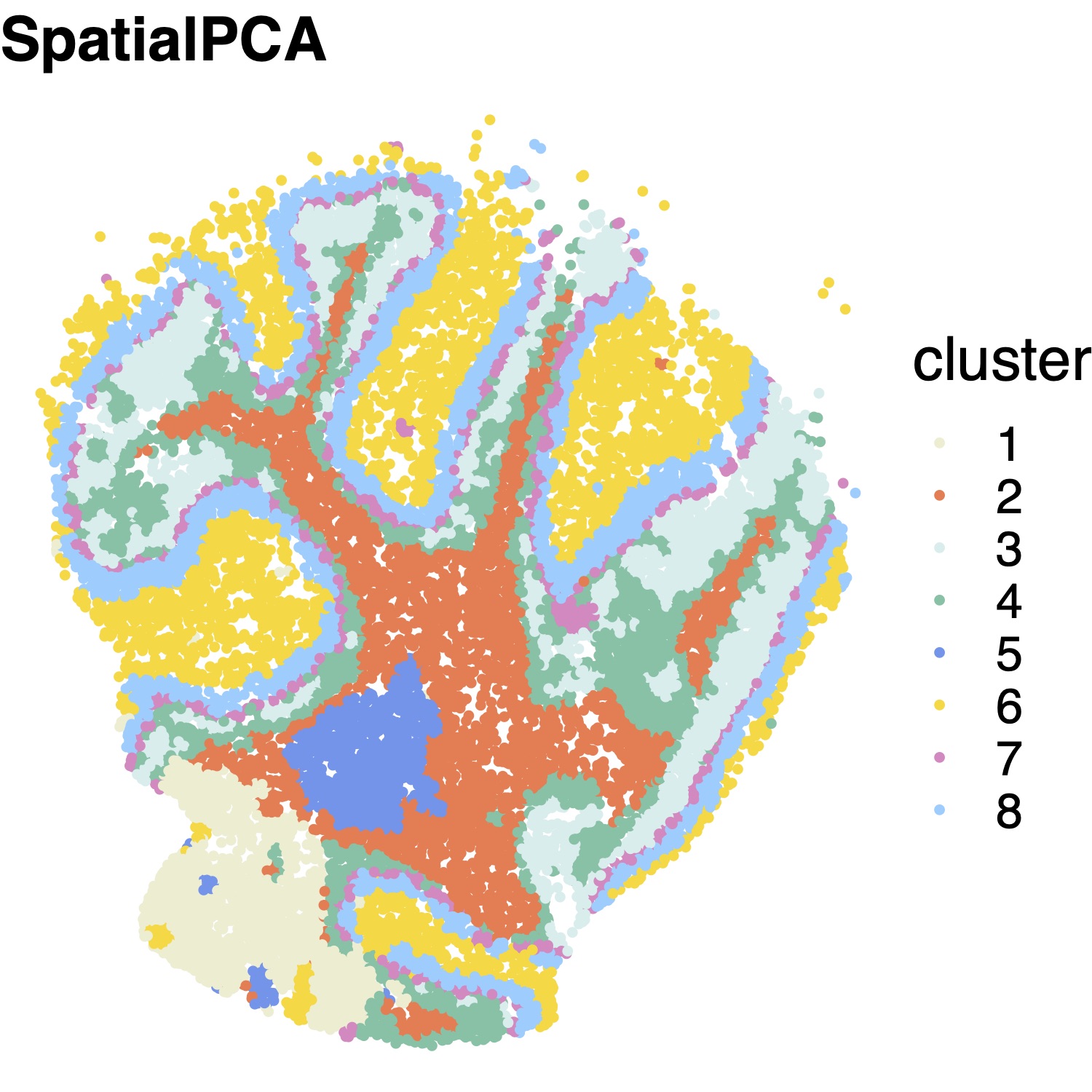
SpatialPCA detects spatial domains through clustering on the spatial PCs. Here we use louvain’s clustering method, which is faster than walktrap method in large sample datasets.
clusterlabel= louvain_clustering(clusternum=8,latent_dat=slideseq@SpatialPCs,knearest=round(sqrt(dim(slideseq@SpatialPCs)[2])) )Spatial domains detected by SpatialPCA.
cbp=c("#9C9EDE" ,"#5CB85C" ,"#E377C2", "#4DBBD5" ,"#FED439" ,"#FF9896", "#FFDC91")
plot_cluster(location=xy_coords,clusterlabel_refine,pointsize=1.5,textsize=20 ,title_in=paste0("SpatialPCA"),color_in=cbp,legend="right")
sessionInfo()R version 4.1.3 (2022-03-10)
Platform: x86_64-pc-linux-gnu (64-bit)
Running under: Ubuntu 18.04.5 LTS
Matrix products: default
BLAS: /usr/lib/x86_64-linux-gnu/openblas/libblas.so.3
LAPACK: /usr/lib/x86_64-linux-gnu/libopenblasp-r0.2.20.so
locale:
[1] LC_CTYPE=en_US.UTF-8 LC_NUMERIC=C
[3] LC_TIME=en_US.UTF-8 LC_COLLATE=en_US.UTF-8
[5] LC_MONETARY=en_US.UTF-8 LC_MESSAGES=en_US.UTF-8
[7] LC_PAPER=en_US.UTF-8 LC_NAME=C
[9] LC_ADDRESS=C LC_TELEPHONE=C
[11] LC_MEASUREMENT=en_US.UTF-8 LC_IDENTIFICATION=C
attached base packages:
[1] stats graphics grDevices utils datasets methods base
other attached packages:
[1] workflowr_1.6.2
loaded via a namespace (and not attached):
[1] Rcpp_1.0.7 whisker_0.4 knitr_1.36 magrittr_2.0.1
[5] R6_2.5.1 rlang_0.4.12 fastmap_1.1.0 fansi_0.5.0
[9] stringr_1.4.0 tools_4.1.3 xfun_0.27 utf8_1.2.2
[13] git2r_0.28.0 jquerylib_0.1.4 htmltools_0.5.2 ellipsis_0.3.2
[17] rprojroot_2.0.2 yaml_2.2.1 digest_0.6.28 tibble_3.1.5
[21] lifecycle_1.0.1 crayon_1.4.1 later_1.3.0 sass_0.4.0
[25] vctrs_0.3.8 promises_1.2.0.1 fs_1.5.0 glue_1.4.2
[29] evaluate_0.14 rmarkdown_2.11 stringi_1.7.5 bslib_0.3.1
[33] compiler_4.1.3 pillar_1.6.4 jsonlite_1.7.2 httpuv_1.6.3
[37] pkgconfig_2.0.3