Below are the example analysis codes for the MOSTA data.
Load package
library(SpatialPCA)

library(reticulate)
library(Seurat)
use_python("/net/mulan/home/shanglu/anaconda3/envs/your_environment/bin/python", required=TRUE) # use your python environment here, I need this to read the h5ad file
sc <- import("scanpy")
library(peakRAM)
library(ggplot2)
Load data
The MOSTA data we used is available at Broad Institute’s single-cell repository. We downloaded one example section named E16.5_E1S3_cell_bin_whole_brain.h5ad.
dataset_name = "E16.5_E1S3"
atlas.data <- sc$read_h5ad("E16.5_E1S3_cell_bin_whole_brain.h5ad")
raw_location = atlas.data$obsm["spatial"]
raw_obs=atlas.data$obs
rawcount = atlas.data$layers["counts"]
rownames(rawcount) <-  atlas.data$obs_names$to_list()
colnames(rawcount) <-  atlas.data$var_names$to_list()
rownames(raw_location) <-  atlas.data$obs_names$to_list()
Run SpatialPCA
rawcount = t(as.matrix(rawcount))
MOSTA = CreateSpatialPCAObject(counts=rawcount, location=raw_location, project = "SpatialPCA",gene.type="spatial",sparkversion="sparkx",numCores_spark=10, gene.number=3000, customGenelist=NULL,min.loctions = 20, min.features=20)
# Variance stabilizing transformation of count matrix of size 18428 by 65303

mem_sparse1 <- peakRAM({
start_time <- Sys.time()
	MOSTA = SpatialPCA_buildKernel(MOSTA, kerneltype="gaussian", bandwidthtype="Silverman",bandwidth.set.by.user=NULL,sparseKernel=TRUE,sparseKernel_tol=1e-5,sparseKernel_ncore=10)
end_time <- Sys.time()
T_sparse1 = end_time - start_time
	MOSTA = SpatialPCA_EstimateLoading(MOSTA,fast=TRUE,SpatialPCnum=20)
end_time <- Sys.time()
T_sparse2 = end_time - start_time
	MOSTA = SpatialPCA_SpatialPCs(MOSTA, fast=TRUE)
end_time <- Sys.time()
T_sparse3 = end_time - start_time
})


# save results
SpatialPCA_result = list()
SpatialPCA_result$SpatialPCs  = as.matrix(MOSTA@SpatialPCs)
SpatialPCA_result$normalized_expr  = MOSTA@normalized_expr
SpatialPCA_result$location = MOSTA@location
save(SpatialPCA_result, file = paste0(dataset_name,"_SpatialPCA_result.RData"))
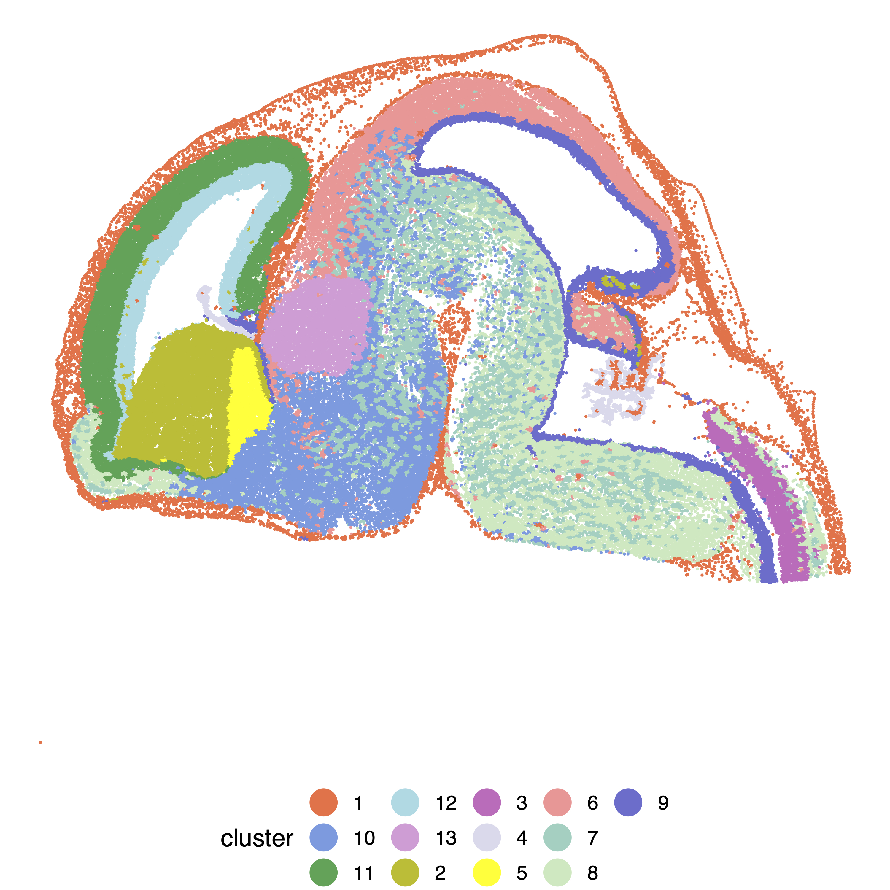
Obtain clustering result
# The original study labeled the tissue section into 17 regions.
# > raw_obs[1,]
#                         Slice    region sim anno n_genes_by_counts total_counts
# CELL.25 E16.5_A3A4_WholeBrain Epidermis    Fibro               324          526
#         annotation
# CELL.25 Fibroblast
# > length(unique(raw_obs$region))
# [1] 17

# so we tried to assign 17 clusters in the louvain clustering
SpatialPCA_louvain = louvain_clustering(clusternum=17,latent_dat=as.matrix(MOSTA@SpatialPCs), knearest=500)
# spatial domain cluster label for each location
SpatialPCA_result$SpatialPCA_louvain_17clusters = SpatialPCA_louvain
save(SpatialPCA_result, file = paste0(dataset_name,"_SpatialPCA_result.RData"))

# we found that a larger number of nearest neighbors (the number is 500 here) will tend to result in better connected/continuou regions, and a smaller number will give you more regions but less connected. You may want to tune the parameters to achieve a better visualization.
s
# Visualize spatial domains detected by SpatialPCA.
cbp_spatialpca = c( "#FD7446" ,"#709AE1", "#31A354","#9EDAE5",
 "#DE9ED6" ,"#BCBD22", "#CE6DBD" ,"#DADAEB" ,
 "yellow", "#FF9896","#91D1C2", "#C7E9C0" ,
 "#6B6ECF", "#7B4173" )

  pdf(paste0("Figure_",dataset_name,"_SpatialPCA_cluster.pdf"),width=10,height=10)
      loc1 = unlist(SpatialPCA_result$location[,1])
      loc2 = unlist(SpatialPCA_result$location[,2])
      cluster = as.character(SpatialPCA_louvain)
      datt = data.frame(cluster, loc1, loc2)
      p = ggplot(datt, aes(x = loc1, y = loc2, color = cluster)) +
        geom_point( alpha = 1,size=0.5) +
        scale_color_manual(values = cbp_spatialpca)+
        theme_void()+
        theme(plot.title = element_text(size = 20,  face = "bold"),
              text = element_text(size = 20),
              #axis.title = element_text(face="bold"),
              #axis.text.x=element_text(size = 15) ,
              legend.position = "bottom")+
        guides(colour = guide_legend(override.aes = list(size=10)))
    print(p)
  dev.off()
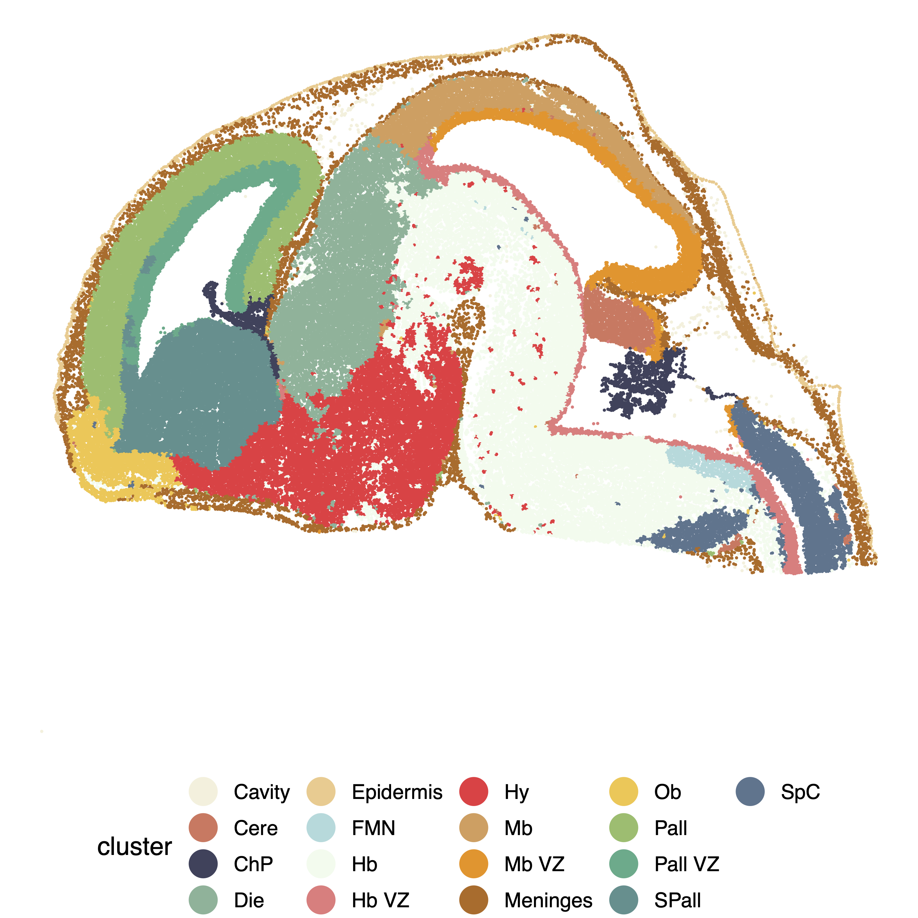
The original region annotation from the data is shown below:
D3=c("#f4f1de","#e07a5f","#3d405b","#81b29a","#f2cc8f","#a8dadc","#f1faee","#f08080",
"#F94144", "#dda15e", "#F8961E" ,"#bc6c25", "#F9C74F" ,"#90BE6D", "#43AA8B",
 "#4D908E", "#577590", "#277DA1", "#AEC7E8" ,"#FFBB78" ,"#98DF8A", "#FF9896",
"#C5B0D5" ,"#C49C94", "#F7B6D2", "#C7C7C7" ,"#DBDB8D" ,"#9EDAE5", "#393B79",
"#637939", "#8C6D31", "#843C39", "#7B4173" ,"#5254A3" ,"#8CA252", "#BD9E39",
"#AD494A", "#A55194", "#6B6ECF", "#B5CF6B", "#E7BA52" ,"#D6616B", "#CE6DBD",
"#9C9EDE", "#CEDB9C" ,"#E7CB94", "#E7969C", "#DE9ED6" ,"#3182BD", "#E6550D",
"#31A354", "#756BB1" ,"#636363", "#6BAED6" ,"#FD8D3C" ,"#74C476", "#9E9AC8",
"#969696", "#9ECAE1" ,"#FDAE6B", "#A1D99B" ,"#BCBDDC" ,"#BDBDBD", "#C6DBEF",
"#FDD0A2" ,"#C7E9C0" ,"#DADAEB", "#D9D9D9")

pdf(paste0("Figure_",dataset_name,"_region.pdf"),width=10,height=10)
      loc1 = unlist(SpatialPCA_result$location[,1])
      loc2 = unlist(SpatialPCA_result$location[,2])
      cluster = as.character(raw_obs$region)
      datt = data.frame(cluster, loc1, loc2)
      p = ggplot(datt, aes(x = loc1, y = loc2, color = cluster)) +
        geom_point( alpha = 1,size=0.5) +
        scale_color_manual(values = D3)+
        theme_void()+
        theme(plot.title = element_text(size = 20,  face = "bold"),
              text = element_text(size = 20),
              #axis.title = element_text(face="bold"),
              #axis.text.x=element_text(size = 15) ,
              legend.position = "bottom")+
        guides(colour = guide_legend(override.aes = list(size=10)))
    print(p)
  dev.off()
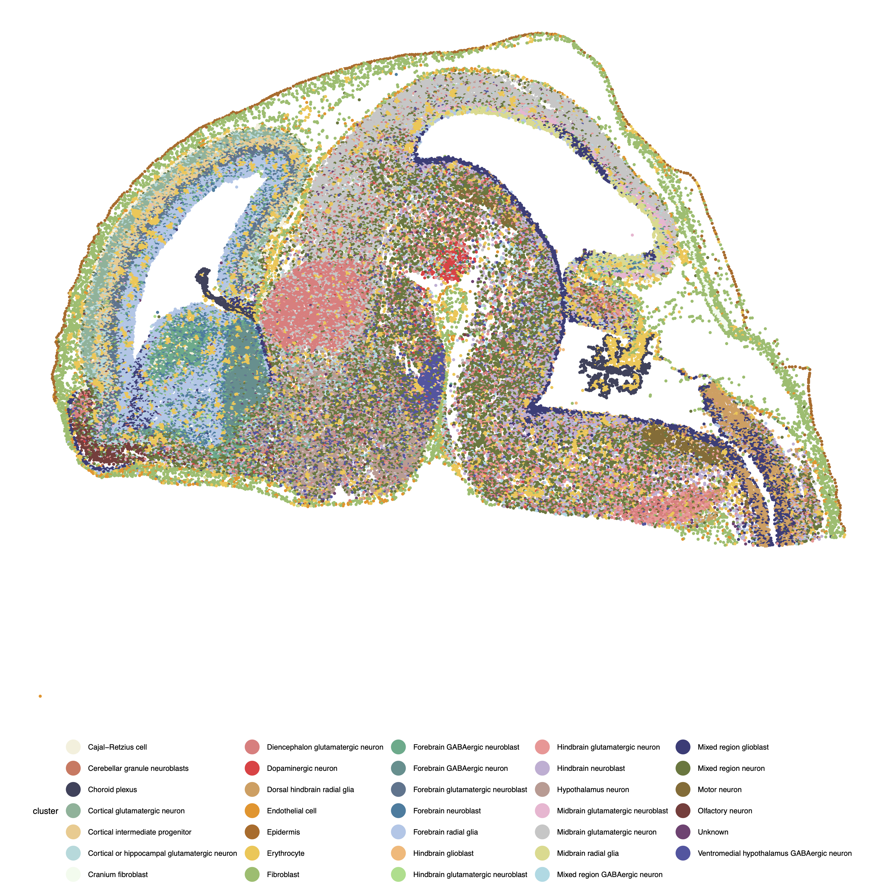
The original cell type annotation from the data is shown below:
  pdf(paste0("Figure_",dataset_name,"_celltype.pdf"),width=10,height=10)
      loc1 = unlist(SpatialPCA_result$location[,1])
      loc2 = unlist(SpatialPCA_result$location[,2])
      cluster = as.character(raw_obs$annotation)
      datt = data.frame(cluster, loc1, loc2)
      p = ggplot(datt, aes(x = loc1, y = loc2, color = cluster)) +
        geom_point( alpha = 1,size=0.5) +
        scale_color_manual(values = D3)+
        theme_void()+
        theme(plot.title = element_text(size = 7,  face = "bold"),
              text = element_text(size = 7),
              #axis.title = element_text(face="bold"),
              #axis.text.x=element_text(size = 15) ,
              legend.position = "bottom")+
        guides(colour = guide_legend(override.aes = list(size=5)))
    print(p)
  dev.off()