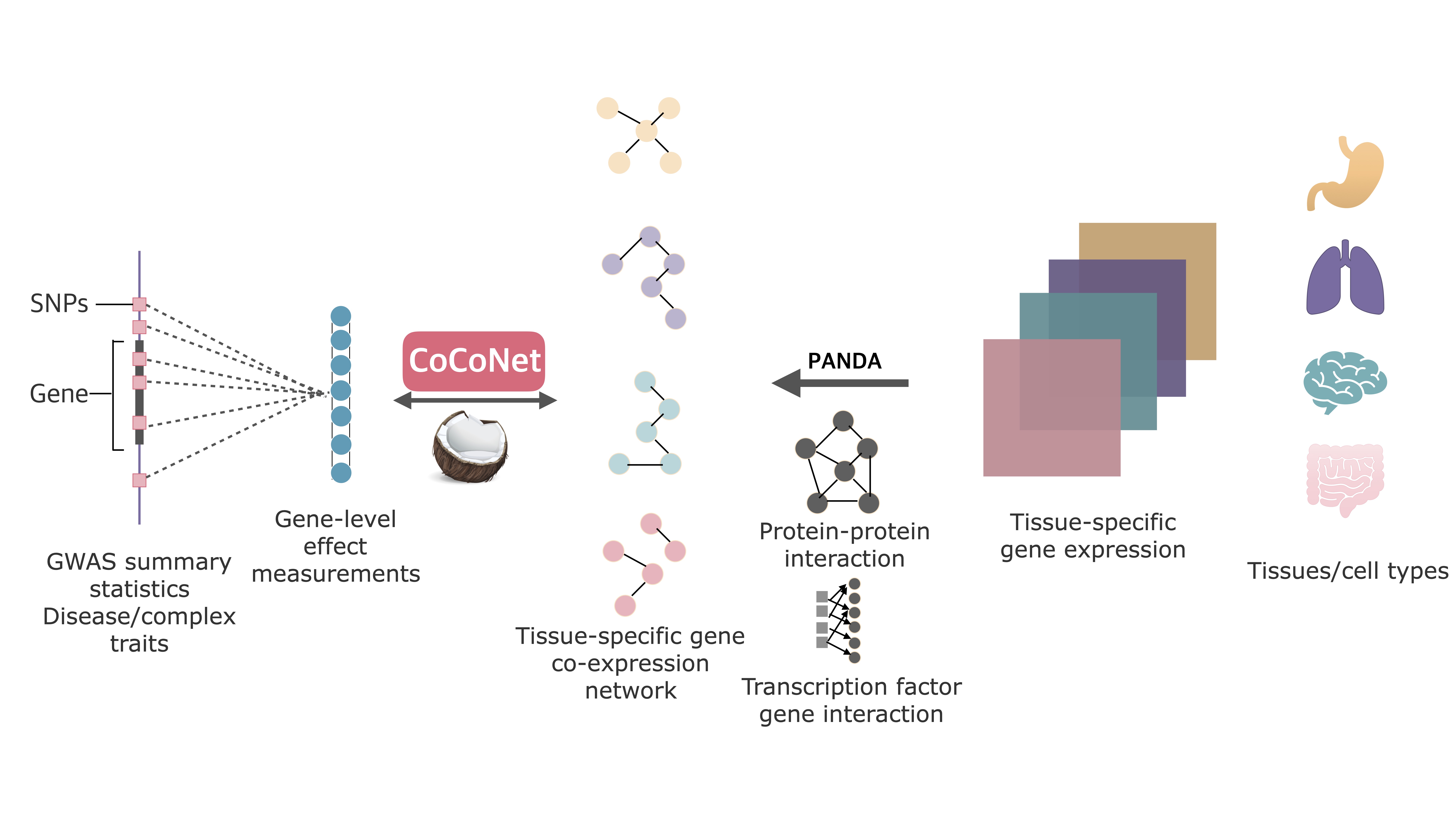
CoCoNet is an efficient method to facilitate the identification of trait-relevant tissues or cell types. We apply CoCoNet for an in-depth analysis of four neurological disorders and four autoimmune diseases, where we integrate the corresponding GWASs with bulk RNAseq data from 38 tissues and single cell RNAseq data from 10 cell types. Our Paper on Plos Genetics: Leveraging Gene Co-expression Patterns to Infer Trait-Relevant Tissues in Genome-wide Association Studies
CoCoNet incorporates tissue-specific gene co-expression networks constructed from either bulk or single cell RNA sequencing (RNAseq) studies with GWAS data for trait-tissue inference. In particular, CoCoNet relies on a covariance regression network model to express gene-level effect sizes for the given GWAS trait as a function of the tissue-specific co-expression adjacency matrix. With a composite likelihood-based inference algorithm, CoCoNet is scalable to tens of thousands of genes.
Install the Package
# (Need to make sure the R package "Rcpp" is already installed.)
# Install devtools if necessary
install.packages('devtools')
# Install CoCoNet
devtools::install_github('xzhoulab/CoCoNet')
# Load the package
library(CoCoNet)

# For windows users:
# Try "install.packages('devtools',type = "win.binary")" if you have problems with installing devtools on windows.
# For mac users:
# This package requires Rcpp and RcppArmadillo as dependencies, which require Xcode or other compilers.
Example: GTEx tissues in GWAS trait BIPSCZ
Load data for GTEx tissue networks and scaled gene level effect sizes, which can be downloaded from this google drive here.
load("tissue_net.RData")
load("tissue_name.RData")
load("outcome_tissue_scale.RData")
In total we have 38 tissues, the network are ordered by the tissue names
> tissue_name
 [1] "Adipose_subcutaneous"      "Adipose_visceral"
 [3] "Adrenal_gland"             "Artery_aorta"
 [5] "Artery_coronary"           "Artery_tibial"
 [7] "Brain_other"               "Brain_cerebellum"
 [9] "Brain_basal_ganglia"       "Breast"
[11] "Lymphoblastoid_cell_line"  "Fibroblast_cell_line"
[13] "Colon_sigmoid"             "Colon_transverse"
[15] "Gastroesophageal_junction" "Esophagus_mucosa"
[17] "Esophagus_muscularis"      "Heart_atrial_appendage"
[19] "Heart_left_ventricle"      "Kidney_cortex"
[21] "Liver"                     "Lung"
[23] "Minor_salivary_gland"      "Skeletal_muscle"
[25] "Tibial_nerve"              "Ovary"
[27] "Pancreas"                  "Pituitary"
[29] "Prostate"                  "Skin"
[31] "Intestine_terminal_ileum"  "Spleen"
[33] "Stomach"                   "Testis"
[35] "Thyroid"                   "Uterus"
[37] "Vagina"                    "Whole_blood"
The first tissue is “Adipose_subcutaneous”, which looks like this:
> tissue_net[[1]][1:4,1:4]
                ENSG00000106546 ENSG00000160224 ENSG00000156150 ENSG00000052850
ENSG00000106546               0               0               0               0
ENSG00000160224               0               0               0               0
ENSG00000156150               0               0               0               0
ENSG00000052850               0               0               0               0
The scaled gene level effect sizes look like this:
> outcome_tissue_scale[1:2,]
                       SCZ        BIP     BIPSCZ  Alzheimer        PBC
ENSG00000106546 -0.4858255 0.08469493  0.3612639  0.3880098 -0.3153474
ENSG00000160224 -0.5557115 1.13772920 -0.6826089 -0.5361030  0.1588954
                        CD        UC        IBD
ENSG00000106546 -0.3582144 0.3233601 -0.2106639
ENSG00000160224  1.5500738 1.4571102  1.5182206
For the first pair of disease and tissue, BIPSCZ - Adipose_subcutaneous:
A = tissue_net[[1]]
start_time = Sys.time()
result = CoCoNet(outcome_tissue_scale[,3], max_path = 1, A)
end_time = Sys.time()
end_time - start_time

# this step takes several minutes, on average 3000M memory.