All of the processed data for the following analysis could be found here.
Section 1: Build cell type specific networks in GTEx single cell dataset.
Set workpath
workpath = "~path/coconet_cell/panda"
Data downloaded from GTEx Portal:
wget https://storage.googleapis.com/gtex_additional_datasets/single_cell_data/GTEx_droncseq_hip_pcf.tar
load needed files
load("~path/outcome_cell_scale.RData")
gene_table = read.table("~path/genetable.txt", header=T)
motif = read.table("~path/pandas/PANDA_for_server/data/motif.txt") # same as in GTEx tissue PANDA input, downloaded from same website
ppi = read.table("~path/pandas/PANDA_for_server/data/ppi.txt") # same as in GTEx tissue PANDA input, downloaded from same website
expr = read.table("~path/single_cell_gtex/GTEx_droncseq_hip_pcf/GTEx_droncseq_hip_pcf.umi_counts.txt",header=T) # GTEx single cell expression
cell_anno = read.csv("~path/single_cell_gtex/GTEx_droncseq_hip_pcf/cell_annotation.csv",header=T) # cell type annotation for GTEx single cell expression

#> dim(expr)
#[1] 32111 14963
#> dim(cell_anno)
#[1] 14963     6
motif is a file of lots of TF-gene pairs, column1: TF names, column2: gene names
the dimension is same as in the PANDA output file PANDA_tissues_regulatory.txt
PANDA_tissues_regulatory.txt contains all edge weights of TF-gene pairs in motif.txt
grch37 for converting HGNC to ENSG ID
library(biomaRt)
grch37 = useMart(biomart="ENSEMBL_MART_ENSEMBL", host="grch37.ensembl.org", path="/biomart/martservice")
listDatasets(grch37)
grch37 = useDataset("hsapiens_gene_ensembl",mart=grch37)
map HGNC ID to ENSG ID, since we are using ENSG IDs in gene effect size file and only keep genes that we already have annotation for TSS TES location
dict = rownames(expr)
HGNC_to_ENSE=getBM(attributes=c('hgnc_symbol','ensembl_gene_id'),
       filters = 'hgnc_symbol',
       values = dict,
       mart = grch37)  # convert gene from  hgnc_symbol to ensembl_gene_id, make dictionary
ENSG_gene_table = as.character(gene_table$ENSG_ID)
index = which(HGNC_to_ENSE$ensembl_gene_id %in% ENSG_gene_table )
dictionary = HGNC_to_ENSE[index,]
dictionary1 = dictionary[-13896,] # the row 13896 is empty
expr_gene = rownames(expr)[match(as.character(dictionary1$hgnc_symbol),rownames(expr) )]
expr_mat = expr[match(as.character(dictionary1$hgnc_symbol),rownames(expr) ),]
Prepare RPKM expression
gene_annotate = match(dictionary1$ensembl_gene_id,as.character(gene_table$ENSG_ID))
l = gene_table$distance[gene_annotate]
cS <- colSums(expr_mat) #Total mapped reads per sample
rpkm <- (10^6)*t(t(expr_mat/l)/cS)
#save(rpkm, file = "rpkm.RData")
double quantile Normalization on log10(rpkm+1)
log10_rpkm = log10(rpkm+1)
GTEx_expr_sc_log10_plus1_gene <- t(apply(log10_rpkm,2, function(x) qqnorm(x, plot=F)$x))
GTEx_expr_sc_log10_plus1_cell <- t(apply(GTEx_expr_sc_log10_plus1_gene,1, function(x) qqnorm(x, plot=F)$x))
GTEx_expr_sc_log10 = t(GTEx_expr_sc_log10_plus1_cell)
#save(GTEx_expr_sc_log10, file = "GTEx_expr_sc_log10.RData")
make cell type annotation. Get cell type index for each cell
sum(colnames(expr_norm)==as.character(cell_anno$Cell_ID))
colnameexpr = gsub(".", '-', as.character(colnames(expr_norm)), fixed = T)
type_in_order = c()
for(i in 1:length(colnames(expr_norm))){
	type_in_order[i] = which(as.character(cell_anno$Cell_ID) %in% colnameexpr[i])
}
cell_type = as.character(cell_anno$Cluster_Name)[type_in_order]
celluniquetype = unique(cell_type)
index_type  = list()
count = 0
for(i in celluniquetype){
	count = count + 1
	index_type[[count]] = which(cell_type == i)
}
calculate gene specificity by cell type
library( matrixStats )
IQR_rpkmlog10_all = unlist(apply(GTEx_expr_sc_log10,1, function(x) IQR(x)))
median_rpkmlog10_all = rowMedians(GTEx_expr_sc_log10)
gene_rpkmlog10_specifity = matrix(0,19822,15)
for(i in 1:15){
	print(i)
	expr_tmp = GTEx_expr_sc_log10[, index_type[[i]]]
  	median_tmp = rowMedians(expr_tmp)
	gene_rpkmlog10_specifity[,i] = (median_tmp-median_rpkmlog10_all)/IQR_rpkmlog10_all
}
m = rowSums(gene_rpkmlog10_specifity)
retained genes with total specificity score in tissues greater than the median value across all genes.
ind = which(m>-2.803) # use median
length(ind)
GTEx_expr_sc = GTEx_expr_sc_log10[ind,]
rownames(GTEx_expr_sc) = dictionary1$hgnc_symbol[ind]
dict9900 = dictionary1[ind,]
make new motif file. In the TF by gene matrix produced by PANDA, if std of any column is 0, it will cause NA in the normalization step, and algorithm won’t work. in other words, we retained genes that are TF factors and have at least one connection to genes we already retained.
genenames = rownames(GTEx_expr_sc)
motif_new = motif[which(as.character(motif$V1) %in% genenames),]
xx=intersect(as.character(motif_new$V2), dict9900$ensembl_gene_id)
motif_use = motif_new[which(as.character(motif_new$V2) %in% xx),]
dict8270 = dict9900[which(dict9900$ensembl_gene_id %in% xx),]
GTEx_expr_sc_8270 = GTEx_expr_sc[which(dict9900$ensembl_gene_id %in% xx),]
need to remove gene with 0 std of i-th column in TF by gene matrix
i=6560
# update files
dict_update = dict8270[-6560,]
GTEx_expr_sc_ensg = 	GTEx_expr_sc_8270[-6560,]
rownames(GTEx_expr_sc_ensg)=dict_update$ensembl_gene_id
motif_update = motif_use[-which(as.character(motif_use$V2)=="ENSG00000211746"),]
make new ppi file
ppi[,1]=as.character(ppi[,1])
ppi[,2]=as.character(ppi[,2])
ind1 = which(ppi[,1] %in% dict_update$hgnc_symbol)
ind2 = which(ppi[,2] %in% dict_update$hgnc_symbol)
ind = intersect(ind1, ind2)
ppi_new = ppi[ind,]
write.table(ppi_new, "ppi_new.txt",  col.names=F, quote=F,row.names=F)
reorder cells, to prepare input expression file for PANDA
tissue_names = c( "ASC1"     ,    "ASC2"   ,      "END"       ,   "GABA1"    ,    "GABA2"       ,
"MG"     ,      "NSC"        ,  "ODC1"       ,  "OPC"    ,      "Unclassified",
"exCA1"     ,   "exCA3"  ,      "exDG"     ,    "exPFC1"    ,   "exPFC2" )

expr_list = list()
count = 0
GTEx_expr_sc_reorder = matrix(0,dim(GTEx_expr_sc_ensg)[1],1)
cell_type_reorder = c()
for(i in tissue_names){
	print(count)
	count = count+1
	col_index = which(cell_type %in% i)
	expr_list[[count]] = GTEx_expr_sc_ensg[,col_index]
	GTEx_expr_sc_reorder = cbind(GTEx_expr_sc_reorder,expr_list[[count]] )
	cell_type_reorder = c(cell_type_reorder,rep(i,dim(expr_list[[count]])[2]))
}
GTEx_expr_sc_reorder = GTEx_expr_sc_reorder[,-1]
my_cell_type_reorder = cbind(colnames(GTEx_expr_sc_reorder), cell_type_reorder)
write.table(GTEx_expr_sc_reorder, "GTEx_expr_sc_reorder.txt",  col.names=F, quote=F)
write.table(motif_update, "motif_update.txt",  col.names=F, quote=F,row.names=F)
write.table(my_cell_type_reorder, "my_cell_type_reorder.txt",  col.names=F, quote=F,row.names=F)
run matlab
matlab codes can be found here: here.
nohup matlab -nodisplay -nodesktop -nojvm -nosplash < RunPANDA.m &
then collect results
% in matlab (faster than in R)
motif_file='motif_update.txt'; % motif prior
exp_file='GTEx_expr_sc_reorder.txt'; % expression data without headers
ppi_file='ppi_new.txt'; %  ppi prior
sample_file='my_cell_type_reorder.txt'; % information on sample order and tissues
fid=fopen(exp_file, 'r');
disp('fid=fopen(exp_file)')
headings=fgetl(fid);
NumConditions=length(regexp(headings, ' '));
%
disp('NumConditions')
frewind(fid);
Exp=textscan(fid, ['%s', repmat('%f', 1, NumConditions)], 'delimiter', ' ', 'CommentStyle', '#');
fclose(fid);
GeneNames=Exp{1};
disp('GeneNames')
NumGenes=length(GeneNames);
disp('NumGenes')
Exp=cat(2, Exp{2:end});
disp('Exp')
%
PANDA_InputEdges = 'PANDA_InputEdges.pairs';
PANDA_weights = 'PANDA_tissues_regulatory.txt'
[TF, gene, weight]=textread(PANDA_InputEdges, '%s%s%f');
disp('PANDA_InputEdges read')
[weight1, weight2, weight3,weight4, weight5, weight6,weight7, weight8, weight9,weight10, weight11, weight12,weight13, weight14, weight15]=textread(PANDA_weights, '%f %f %f %f %f %f %f %f %f %f %f %f %f %f %f ');
disp('PANDA_weights read')
TFNames=unique(TF);
disp('TFNames')
NumTFs=length(TFNames);
[~,i]=ismember(TF, TFNames);
[~,j]=ismember(gene, GeneNames);
%
RegNet=zeros(NumTFs, NumGenes);
RegNet(sub2ind([NumTFs, NumGenes], i, j))=weight1;
save('RegNet1.mat','RegNet')
% do above for 1-15 tissues
save('TF_gene_names.mat','TFNames','GeneNames')
go back to R
library(R.matlab)
TF_gene_names = readMat("TF_gene_names.mat")
i=1
for(i in 1:15){
print(i)
Test_data = readMat(paste0("RegNet",i,".mat"))
TF_gene_mat = Test_data$RegNet
colnames(TF_gene_mat) = unlist(TF_gene_names$GeneNames)
rownames(TF_gene_mat) = unlist(TF_gene_names$TFNames)	# gene symbol
rownames(TF_gene_mat) = dict8269$ensembl_gene_id[which(dict8269$hgnc_symbol %in% rownames(TF_gene_mat))]# gene ENSG id
mat1 = matrix(0,dim(TF_gene_mat)[2],dim(TF_gene_mat)[2])
mat2 = matrix(0,dim(TF_gene_mat)[2],dim(TF_gene_mat)[2])
TF_gene_mat = (TF_gene_mat>0)
mat1[which(colnames(TF_gene_mat) %in% rownames(TF_gene_mat)),]=TF_gene_mat
mat2[,which(colnames(TF_gene_mat) %in% rownames(TF_gene_mat))]=t(TF_gene_mat)
mat = mat1+mat2
mat[mat>0]=1
rownames(mat) = colnames(TF_gene_mat)
colnames(mat) = colnames(TF_gene_mat)
save(mat, file = paste0("Coconet_cell_",i,".RData"))
}


# above is weighted network, make it symmetric and binary
load(paste0("Coconet_cell_",i,".RData"))
mat = Matrix::forceSymmetric(mat)
mat = (mat>0)*1
diag(mat)=0
Section 2: tissue-specific network construction
For the tissue-specific network construction, we used the result from this paper: Understanding Tissue-Specific Gene Regulation
This paper reconstructed networks from panda, built Gene regulatory networks for 38 human tissues. All needed data can be found here.
First check how many genes in GTEx_PANDA_tissues.RData overlap with our gene level effect sizes extracted from summary statistics.
load("GTEx_PANDA_tissues.RData")
# annotate genes with grch37
library(biomaRt)
grch37 = useMart(biomart="ENSEMBL_MART_ENSEMBL", host="grch37.ensembl.org", path="/biomart/martservice")
listDatasets(grch37)
grch37 = useDataset("hsapiens_gene_ensembl",mart=grch37)
# extract genes overlapped with 49015 genes in summary statistics
load("~/path/Sigma_pop_traits.RData")
gene_table = read.table("~/path/genetable.txt", header=T)
TF = as.character(edges$TF)
dict = unique(TF) # make dictionary
HGNC_to_ENSE=getBM(attributes=c('hgnc_symbol','ensembl_gene_id'),
       filters = 'hgnc_symbol',
       values = dict,
       mart = grch37)
ENSG_gene_table = as.character(gene_table$ENSG_ID)
index = which(HGNC_to_ENSE$ensembl_gene_id %in% ENSG_gene_table )
dict = HGNC_to_ENSE[index,]
get edges with both genes exist in ENSG_gene_table
# filter genes in first column
index_col_1 = which(as.character(edges$TF) %in% as.character(dict$hgnc_symbol) )
# filter genes in second column
ENSG_gene_table = as.character(gene_table$ENSG_ID)
index_col_2 = which(as.character(edges$Gene) %in% ENSG_gene_table )
index_col_edge = intersect(index_col_1, index_col_2)
filter genes by specificity in tissues
net_specific = rowSums(netTS)
index_specific = which(net_specific>0)
index_specific_col = intersect(index_specific, index_col_edge)
exp_specific = rowSums(expTS)
gene_expr_ge = as.character(genes$Name[which(exp_specific>1)])
index_gene_expr_ge = which(as.character(edges$Gene) %in% gene_expr_ge)
index_specific = which(net_specific>0)
index_specific_col = intersect(index_specific, index_col_edge)
ind = intersect(index_gene_expr_ge, index_specific_col)
use_gene = unique(as.character(edges$Gene)[ind])
use_edges = edges[ind,]
use_net = net[ind,]
all_gene = unique(c(as.character(dict$ensembl_gene_id),as.character(use_edges$Gene)))

#> length(all_gene)
#[1] 5359

save(all_gene, file = "all_gene.RData")
save(use_net,file = "use_net.RData")
save(use_edges,file = "use_edges.RData")
get gene effect sizes for 5359 genes
tissue_name = colnames(use_net)
save(tissue_name, file = "tissue_name.RData")
gene_tsn = all_gene
save(gene_tsn, file = "gene_tsn.RData")
ENSG_gene_table = as.character(gene_table$ENSG_ID)
indexk = NULL
for(k in 1:length(all_gene)){
	indexk[k] = which(ENSG_gene_table %in% all_gene[k])
}

sigma_sona = Sigma_pop_traits[indexk,]
rownames(sigma_sona) = gene_tsn
save(sigma_sona, file = "outcome_tissue.RData")
Build network using edge information
# this part of R code can be slow, better to refer to the single cell process procedures and use matlab
name1 = as.character(use_edges$TF)
name2 = as.character(use_edges$Gene)
index1 = NULL
index2 = NULL
weightindex = NULL
for(i in 1:length(name1)){
if(length(which(dict$hgnc_symbol %in% name1[i]))>0){
name1_ensg = as.character(dict$ensembl_gene_id)[which(dict$hgnc_symbol %in% name1[i])]
index1[i] = which(all_gene %in% name1_ensg)
index2[i] = which(all_gene %in% name2[i])
}
}
index_dat = data.frame(index1, index2)
save(index_dat, file = "index_dat.RData")

for(j in 1:38){
print(j)
mat = matrix(0, length(all_gene), length(all_gene))
for(xx in 1:length(index1)){
	mat[index1[xx],index2[xx]]=use_net[xx,j]
}
save(mat, file = paste0("mat_weighted_tissue_",j,".RData"))

}

# above is weighted network, make it symmetric and binary
load(paste0("mat_weighted_tissue_",j,".RData"))
mat = Matrix::forceSymmetric(mat)
mat = (mat>0)*1
diag(mat)=0
Section 3: gene effect size estimation
With SNP-level GWAS summary statistics and LD information from the reference panel, we obtained gene-level heritability estimates using MQS. We scaled the gene-level heritability estimates by the number of SNPs in each gene.
The sumstat.meta file could be downloaded from gene_effect_size_generate folder here.
The genetable.txt could be downloaded from here.
snp=read.csv("~/effectsize/data/sumstat.meta",header=T,sep=" ")
gene=read.csv("~/effectsize/data/genetable.txt",header=T,sep="\t")
#seperate snp and gene according to chromosome number
for (name in levels(as.factor(snp$CHR))){
  tmp=subset(snp,CHR==name)
  fn=paste('snp_chr_',gsub(' ','',name),".txt",sep='')
  write.csv(tmp,fn,row.names=FALSE)
}
for (name in levels(as.factor(gene$chr))){
  tmp=subset(gene,chr==name)
  fn=paste('gene_chr_',gsub(' ','',name),".txt",sep='')
  write.csv(tmp,fn,row.names=FALSE)
}
Get -/+1MB snps, snps in genes have no overlap
chr_gene_index2=NULL
for(chr_id in 1:22) {

  gmap <- read.table(paste0("~/effectsize/Analysis/gene_snp_chr/gene_chr_", chr_id, ".txt"), sep = ",", header = T)
  smap <- read.table(paste0("~/effectsize/Analysis/gene_snp_chr/snp_chr_", chr_id, ".txt"), sep = ",", header = T)[, c(1, 2, 3)]
  num_gene <- dim(gmap)[1]
  snp_index <- NULL
  genmap <- NULL
  block_num <- 0
  count=0

  for(i in 1:num_gene) {

    snp_start <- gmap[i, 3] - 1000000
    snp_end <- gmap[i, 4] + 1000000
    dis_to_lastgene=abs(smap[, 3]-gmap[i-1, 3])
    dis_to_currentgene=abs(smap[, 3]-gmap[i, 3])
    dis_to_nextgene=abs(smap[, 3]-gmap[i+1, 3])

    temp_index <- which(smap[, 3] >= snp_start &  smap[, 3] <= snp_end & dis_to_currentgene<dis_to_lastgene &dis_to_currentgene<dis_to_nextgene)
    if(length(temp_index) < 20) {
      cat("There is no enough SNP in   ", i, "   gene", fill = T)
      next
    } else {
      count=count+1
      snp_index <- rbind(snp_index, temp_index[c(1, length(temp_index))])
      genmap <- rbind(genmap, gmap[i, ])
      block_num <- block_num + 1
      cat("There are",  length(temp_index), " SNPs in   ", i, "   gene", fill = T)
    }
    fn=paste0("~/effectsize/Analysis/snplist_gene/chr_", chr_id, "_gene_",count,".snpname", sep = "")
    chr_gene_index2=c(chr_gene_index2,i)
    #write.table(smap[temp_index,1], file=fn, quote = F, row.names = F, col.names = F)

  }
  colnames(snp_index) <- c("snp_start", "snp_end")
  write.table(snp_index, paste("~/effectsize/Analysis/OneMB_snp/chr_", chr_id, ".index", sep = ""), quote = F, row.names = F, col.names = T)
  write.table(genmap, paste("~/effectsize/Analysis/OneMB_snp/chr_", chr_id, ".genmap", sep = ""), quote = F, row.names = F, col.names = T)
  write.table(count,paste("~/effectsize/Analysis/OneMB_snp/chr_", chr_id, ".num", sep = ""), quote = F, row.names = F, col.names = F)
  }
get gene table
chr_gene_index1=NULL
chr_gene_index2=NULL
for(i in 1:22){
chr_num=read.table(paste0("~/effectsize/Analysis/OneMB_snp/chr_", i, ".num"),header=F)$V1
chr_gene_index2=c(chr_gene_index2,1:chr_num)
chr_gene_index1=c(chr_gene_index1,rep(i,chr_num))
}

chrlist=list()
for(i in 1:22){
  chrlist[[i]]= read.table(paste0("~/effectsize/Analysis/OneMB_snp/chr_",i,".genmap"),header=T)
  chrgnum=read.table(paste0("~/effectsize/Analysis/OneMB_snp/chr_",i,".num"))$V1
  geneID=NULL
  for(j in 1:chrgnum){
    geneID[j]=strsplit(as.character(chrlist[[i]][,6]), "[.]")[[j]][1]
  }
  index_match=c(1:chrgnum)
  chrlist[[i]]=cbind(chrlist[[i]][,c(1,2,3,4)],geneID,index_match)
}
m=do.call(rbind,chrlist)
Build Genotype matrix:
library(BEDMatrix)
chr_bed=NULL
for(i in 1:length(chr_gene_index1)){
 bed=BEDMatrix(paste0("~/effectsize/Analysis/plink_files/chr_",chr_gene_index1[i],"_gene_",chr_gene_index2[i],".bed"))
 chr_bed=cbind(chr_bed,bed[,])
}
dim(chr_bed)
Make plink usable
chmod u+x ~/effectsize/Analysis/plink2
use plink to extract SNPs corresponding to each gene
#!/bin/bash
#SBATCH --job-name=plink
#SBATCH --mem=20000
#SBATCH --array=1-22
#SBATCH --output=~/effectsize/Analysis/plink_files/out/plink%a.out
#SBATCH --error=~/effectsize/Analysis/plink_files/err/plink%a.err

bash

let k=0

for ((i=1; i<=1000; i++)); do
let k=${k}+1
if [ ${k} -eq ${SLURM_ARRAY_TASK_ID} ]; then
Gfile=~/task1/refgeno/refEUR/ping_chr_${k}
gnum=`cat ~/effectsize/Analysis/OneMB_snp/chr_${i}.num`
for ((j=1; j<=${gnum}; j++)); do
snplist=~/effectsize/Analysis/snplist_gene/chr_${i}_gene_${j}.snpname
./plink2 --bfile ${Gfile} --extract ${snplist} --make-bed --out chr_${i}_gene_${j}
rm *log
rm *nosex
done
fi
done
Use gemma to get per-SNP heritability
# note:
# mkdir gemma_files/output/SCZ..., output files into seperate folders for 8 traits
gemma codes
#!/bin/bash
#SBATCH --job-name=goodluck_gemma
#SBATCH --mem=50000
#SBATCH --array=1-22
#SBATCH --output=~/effectsize/Analysis/gemma_files/out/gemma%a.out
#SBATCH --error=~/effectsize/Analysis/gemma_files/err/gemma%a.err

bash

GEMMA=~/effectsize/task1/SummaryData/gemma
INPATH1=~/effectsize/task1/sumstat
INPATH2=~/effectsize/Analysis/plink_files

let k=0
for ((i=1; i<=100; i++)); do
	let k=${k}+1
	if [ ${k} -eq ${SLURM_ARRAY_TASK_ID} ]; then
		for TRAIT in SCZ BIP BIPSCZ Alzheimer PBC UC CD IBD; do
				gnum=`cat ~/effectsize/Analysis/OneMB_snp/chr_${i}.num`
				BETAFILE=${INPATH1}/${TRAIT}.sumstats
			for ((j=1; j<=${gnum}; j++)); do
				BFILE=${INPATH2}/chr_${i}_gene_${j}
				${GEMMA} -beta ${BETAFILE} -bfile ${BFILE} -c pop.txt -vc 1 -o ${TRAIT}/chr_${i}_gene_${j}
done
done
fi
done
Extract per-SNP heritability
Traits_name=c( "SCZ", "BIP", "BIPSCZ",  "Alzheimer","PBC", "CD", "UC", "IBD")

Sigma2_traits=matrix(0,49015,8)
count=0
for( k in Traits_name){
print(k)
count=count+1
sigma2=NULL
numchr=NULL
SIGMA2=NULL

for(i in 1:22){
			print(i)
  			numchr=read.table(paste0('~/effectsize/Analysis/OneMB_snp/chr_',i,'.num'))$V1
                       for(j in 1:numchr){
                         memo=paste0("~/effectsize/Analysis/gemma_files/output/",k,"/chr_",i,"_gene_",j)
                         gemma.res=read.delim(paste0(memo, ".log.txt", sep=""), head=FALSE)
                         sigma2=as.numeric(unlist(strsplit(as.character(gemma.res[17, ]), "  "))[2])
                         SIGMA2=c(SIGMA2,sigma2)
                       }
}
Sigma2_traits[,count]=SIGMA2
}
colnames(Sigma2_traits)=Traits_name
#want SNP number per gene and se(sigma2)
Sigma2_traits=matrix(0,49015,8)
Sigma2_se_traits=matrix(0,49015,8)
PVE_Traits=matrix(0,49015,8)
PVE_se_Traits=matrix(0,49015,8)

Traits_name = c( "SCZ", "BIP", "BIPSCZ",  "Alzheimer","PBC", "CD", "UC", "IBD")
count=0
for( k in Traits_name){
print(k)
count=count+1
sigma2=NULL
sigma2_se=NULL
pve=NULL
pve_se=NULL
snpnum=NULL
numchr=NULL
SIGMA2=NULL
SIGMA2_SE=NULL
SNPNUM=NULL
PVE=NULL
PVE_SE=NULL
for(i in 1:22){
			print(i)
  			numchr=read.table(paste0('~/effectsize/Analysis/OneMB_snp/chr_',i,'.num'))$V1
                       for(j in 1:numchr){
                         memo=paste0("~/effectsize/Analysis/gemma_files/output/",k,"/chr_",i,"_gene_",j)
                         gemma.res=read.delim(paste0(memo, ".log.txt", sep=""), head=FALSE)
                         #sigma2=as.numeric(unlist(strsplit(as.character(gemma.res[17, ]), "  "))[2])
                         pve=as.numeric(unlist(strsplit(as.character(gemma.res[15, ]), "  "))[2])
                         pve_se=as.numeric(unlist(strsplit(as.character(gemma.res[16, ]), "  "))[2])
                         #sigma2_se=as.numeric(unlist(strsplit(as.character(gemma.res[18, ]), "  "))[2])
                         snpnum=read.table(paste0(memo, ".size.txt", sep=""), head=FALSE)$V1[1]
                         #SIGMA2=c(SIGMA2,sigma2)
                         #SIGMA2_SE=c(SIGMA2_SE,sigma2_se)
                         PVE=c(PVE,pve)
                         PVE_SE=c(PVE_SE,pve_se)
                         SNPNUM=c(SNPNUM,snpnum)
                       }
}
PVE_Traits[,count]=PVE
PVE_se_Traits[,count]=PVE_SE
}
colnames(PVE_Traits)=Traits_name
colnames(PVE_se_Traits)=Traits_name

rownames(PVE_Traits)=m$geneID
rownames(PVE_se_Traits)=m$geneID
Section 4: Figures for CoCoNet method
I used the theme_Publication, scale_fill_Publication, and scale_colour_Publication, the three functions in ggplot theme for publication ready Plots.
library(ggplot2)
library(gridExtra)
theme_Publication <- function(base_size=14, base_family="helvetica") {
# please see the above link for the full functions
...
}
scale_fill_Publication <- function(...){
...
}
scale_colour_Publication <- function(...){
...
}
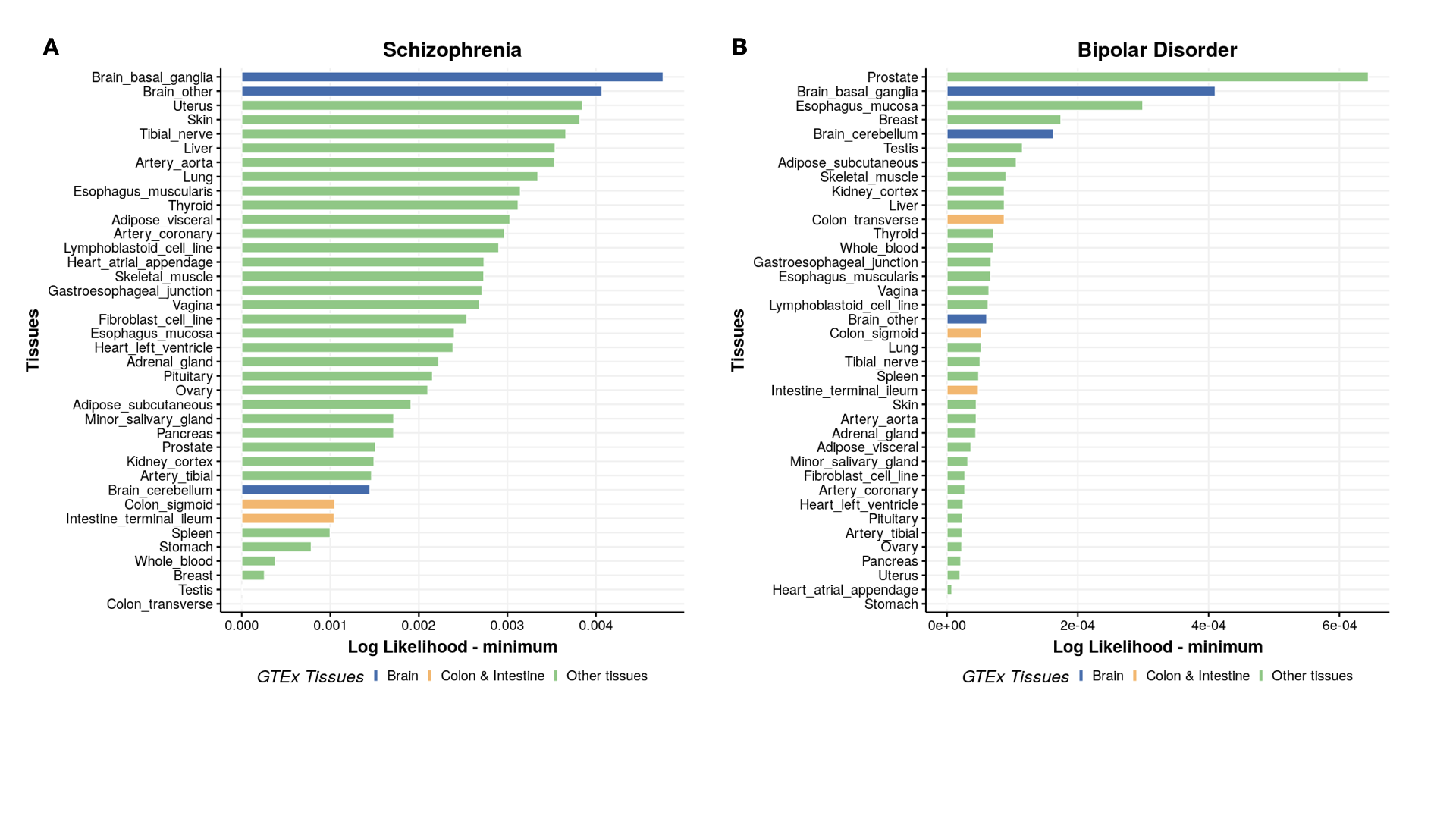
Plot ranking of likelihoods
Plot ranking of tissues
#----------------------
# Tissue likelihood ranking
#----------------------

library(cowplot)
library(ggplot2)
library(gridExtra)
library(ggpubr)

trait_current = c(1:8)
myarr=c( "SCZ","BIP", "BIPSCZ" ,"Alzheimer" , "PBC", "CD" , "UC","IBD"   )
disease_name = c("Schizophrenia","Bipolar Disorder","Bipolar Disorder/Schizophrenia","Alzheimer's Disease","Primary biliary cholangitis","Crohn's Disease","Ulcerative colitis","Inflammatory bowel disease")


dat = list()
p = list()
count = 0
for(j in trait_current){
count = count + 1
lik_expon = c()
	for(tissue in 1:38){
	load(paste0("~path/result/Tissue_trait_",j,"_tissue_",tissue,".RData"))
		re_expon=res1
		lik_expon[tissue] = re_expon$value
	}

trait = myarr[j]
Tissues = as.factor(tissue_name)
Tissues_name = tissue_name
index = c(1:38)
tissue_color = rep(NA,38)
tissue_color[7:9] = "Brain"
tissue_color[c(13,14,31)] = "Colon & Intestine"
tissue_color[-c(7:9,13,14,31 )]="Other tissues"
lik_expon_minus_mean = lik_expon - mean(lik_expon)
ranking = rank(lik_expon_minus_mean)
mydata = data.frame( ranking, h_expon,lik_expon,Tissues_name,index,tissue_color,lik_expon_minus_mean)
mydata$lik_expon = -mydata$lik_expon # this depends on the outcome of the coconet function is likelihood or -likelihood
mydata$lik_min = mydata$lik_expon - min(mydata$lik_expon)
mydata$Trait = rep(myarr[j],dim(mydata)[1])

dat[[count]] =  mydata
p[[count]] = ggbarplot(mydata, x = "Tissues_name", y = "lik_min",
          fill = "tissue_color",           # change fill color by mpg_level
          color = "white",            # Set bar border colors to white
          palette = "jco",            # jco journal color palett. see ?ggpar
          sort.val = "asc",          # Sort the value in descending order
          sort.by.groups = FALSE,     # Don't sort inside each group
          x.text.angle = 90,          # Rotate vertically x axis texts
          ylab = "Log Likelihood - minimum",
          xlab = "Tissues",
          legend.title = "GTEx Tissues",
          rotate = TRUE,
          ggtheme = theme_minimal(),
          title = disease_name[count]
          )
}

k=0
# Repeat codes below:

k=k+1
tiff(paste0("Tissue_",myarr[k],".tiff"), units="in",width=10, height=10,  res=100)
grid.arrange((p[[k]] + scale_fill_Publication() +theme_Publication()),nrow=1)
dev.off()
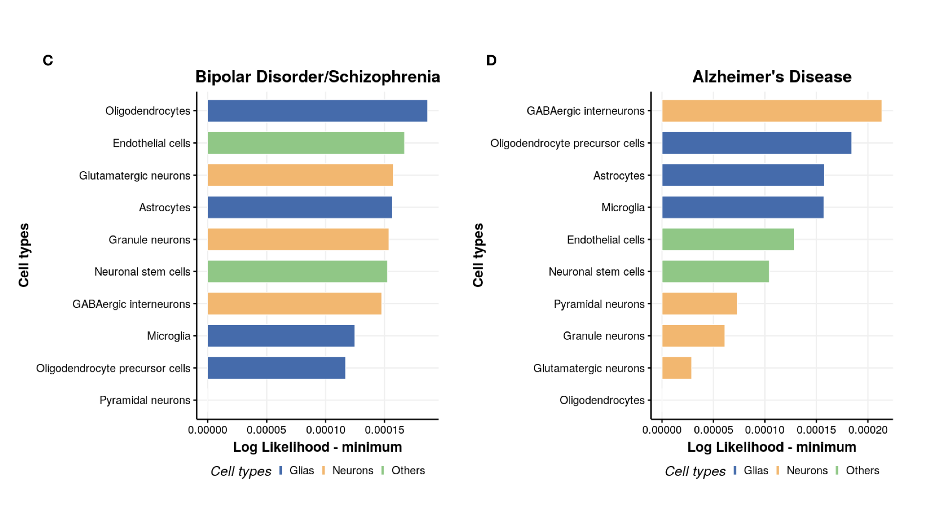
Plot ranking of cell types
#----------------------
# Cell likelihood ranking
#----------------------


cell_type =  c("Astrocytes","Endothelial cells","GABAergic interneurons","Microglia","Neuronal stem cells",
"Oligodendrocytes","Oligodendrocyte precursor cells","Pyramidal neurons","Granule neurons","Glutamatergic neurons")
p <- list()
count=0
dat=list()
for(j in c(1:4)){
count=count+1
lik_expon = c()
	for(tissue in 1:10){
		load(paste0("~path/result/cell_trait_",j,"_tissue_",tissue,".RData"))
		re_expon = res1
		lik_expon[tissue] = re_expon$value
	}
h_expon = h_expon
lik_expon = lik_expon
trait = myarr[j]
Tissues = as.factor(cell_type)
Tissues_name = cell_type
index = c(1:10)
tissue_color = rep(NA,10)
tissue_color[c(1,4,6,7)] = "Glias"
tissue_color[c(2,5)] = "Others"
tissue_color[c(3,8,9,10)] = "Neurons"
lik_expon_minus_mean = lik_expon - mean(lik_expon)
mydata = data.frame(h_expon,lik_expon,Tissues_name,index,tissue_color,lik_expon_minus_mean)
mydata$ranking = rank(mydata$lik_expon)
mydata$lik_expon = -mydata$lik_expon
mydata$lik_min = mydata$lik_expon - min(mydata$lik_expon)
mydata$Trait = rep(myarr[j],dim(mydata)[1])

dat[[count]] =  mydata
p[[count]] = ggbarplot(mydata, x = "Tissues_name", y = "lik_min",
          fill = "tissue_color",           # change fill color by mpg_level
          color = "white",            # Set bar border colors to white
          palette = "jco",            # jco journal color palett. see ?ggpar
          sort.val = "asc",          # Sort the value in descending order
          sort.by.groups = FALSE,     # Don't sort inside each group
          x.text.angle = 90,          # Rotate vertically x axis texts
          ylab = "Log Likelihood - minimum",
          xlab = "Cell types",
          legend.title = "Cell types",
          rotate = TRUE,
          ggtheme = theme_minimal(base_size=25),
          title = disease_name[count]
          )

}

k=0
# Repeat codes below:

k=k+1
tiff(paste0("Cell_",myarr[k],".tiff"), units="in",width=8, height=8,  res=100)
grid.arrange((p[[k]] + scale_fill_Publication() +theme_Publication()),nrow=1)
dev.off()
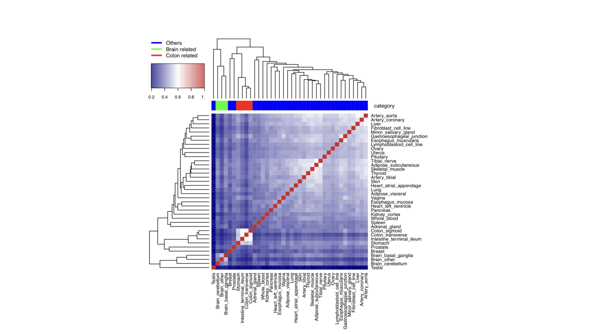
Plot heatmap of tissues measured by Jaccard Index
library(BiRewire)
library(corrplot)
library(heatmap3)

#---------------------------------
# Tissues
#---------------------------------

load("tissue_net.RData")
load("tissue_name.RData")
Tissue_network = tissue_net

# calculate Jaccard Index between each pair of tissues

a = matrix(0,38,38)
for(i in 1:38){
	for(j in (i+1):38){
		a[i,j] = birewire.similarity( Tissue_network[[i]],Tissue_network[[j]])
		a[j,i] = a[i,j]
	}
	print(i)
	print(a[i,])
}
colnames(a) = tissue_name
rownames(a) = tissue_name

# use heatmap3
mapDrugToColor<-function(annotations){
    colorsVector = ifelse(annotations["category"]=="Others",
        "blue", ifelse(annotations["category"]=="Brain related",
        "green", "red"))
    return(colorsVector)
}
testHeatmap3<-function(logCPM, annotations) {
    sampleColors = mapDrugToColor(annotations)

    # Assign just column annotations
    heatmap3(logCPM, margins=c(16,16), ColSideColors=sampleColors,scale="none")
    # Assign column annotations and make a custom legend for them
    heatmap3(logCPM, margins=c(16,16), ColSideColors=sampleColors, scale="none",
        legendfun=function()showLegend(legend=c("Others",
        "Brain related", "Colon related"), col=c("blue", "green", "red"), cex=1))

    # Assign column annotations as a mini-graph instead of colors,
    # and use the built-in labeling for them
    ColSideAnn<-data.frame(Drug=annotations[["category"]])
    heatmap3(logCPM,ColSideAnn=ColSideAnn,
        ColSideFun=function(x)showAnn(x),
        ColSideWidth=0.8)
}
category = c(rep("Others",6),rep("Brain related",3),rep("Others",3),"Colon related",
"Colon related", rep("Others",16),"Colon related","Others","Colon related",rep("Others",5))
gAnnotationData = data.frame(tissue_name, category)
gLogCpmData = a
pdf("Tissue_GTEx_heatmap_unscaled.pdf",width=7, height=7)
diag(gLogCpmData)=1
testHeatmap3(gLogCpmData, gAnnotationData)
dev.off()
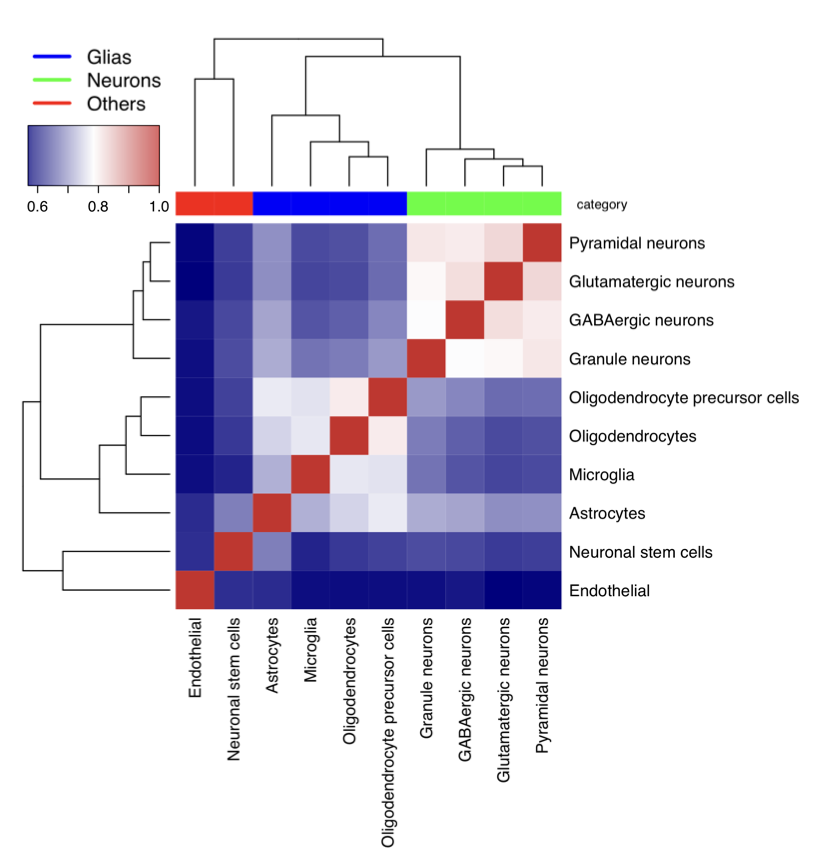
Plot heatmap of cell types measured by Jaccard Index
#---------------------------------
# Cells - same cell type combined
#---------------------------------
load("cell_net.RData")
Tissue_network_cell = cell_net
cell_types =  c("ASC","END","GABA","MG","NSC","ODC","OPC","exCA","exDG","exPFC")
cellnames = c("Astrocytes","Endothelial","GABAergic neurons","Microglia","Neuronal stem cells","Oligodendrocytes","Oligodendrocyte precursor cells","Pyramidal neurons","Granule neurons","Glutamatergic neurons")
category = c("Glias","Endothelial","Neurons","Glias","Neuronal Stem","Glias","Glias","Neurons","Neurons","Neurons")
a = matrix(0,10,10)
for(i in 1:10){
	for(j in (i+1):10){
		a[i,j] = birewire.similarity( Tissue_network_cell[[i]],Tissue_network_cell[[j]])
		a[j,i] = a[i,j]
	}
	print(i)
	print(a[i,])
}
colnames(a) = cellnames
rownames(a) = cellnames
diag(a)=1
mapDrugToColor<-function(annotations){
    colorsVector = ifelse(annotations["category"]=="Glias",
        "blue", ifelse(annotations["category"]=="Neurons",
        "green", "red"))
    return(colorsVector)
}
testHeatmap3<-function(logCPM, annotations) {
    sampleColors = mapDrugToColor(annotations)
    # Assign just column annotations
    heatmap3(logCPM, margins=c(16,16), ColSideColors=sampleColors,scale="none")
    # Assign column annotations and make a custom legend for them
    heatmap3(logCPM, margins=c(16,16), ColSideColors=sampleColors, ,scale="none",
        legendfun=function()showLegend(legend=c("Glias",
        "Neurons", "Others"), col=c("blue", "green", "red"), cex=1.5))

    # Assign column annotations as a mini-graph instead of colors,
    # and use the built-in labeling for them
    ColSideAnn<-data.frame(Drug=annotations[["category"]])
    heatmap3(logCPM,ColSideAnn=ColSideAnn,
        ColSideFun=function(x)showAnn(x),
        ColSideWidth=0.8)
}
gAnnotationData = data.frame(cell_types, category)
gLogCpmData = a
pdf("scGTEx_heatmap_combine_unscaled.pdf",width=7, height=7)
diag(gLogCpmData)=1
testHeatmap3(gLogCpmData, gAnnotationData)
dev.off()
Plot ranking of tissues
Plot ranking of cell types
Heatmap of Jaccard index for tissues / cell types
Heatmap of Jaccard index for cell types
Section 5: Pubmed search results
We partially validated the identified trait-relevant tissue/cell types for the GWAS diseases by searching PubMed, by following this paper.
library(RISmed)

#-------------------------------
#  GTEx Tissue
#-------------------------------

tissues_name = c(
"adipose subcutaneous",      "adipose visceral",
"adrenal gland"  ,           "artery aorta"  ,
"artery coronary",           "artery tibial"     ,
"brain other",               "brain cerebellum"  ,
"brain basal ganglia"    ,   "breast"    ,
"lymphoblastoid cell line" , "fibroblast cell line"   ,
"colon sigmoid"      ,       "colon transverse"  ,
"gastroesophageal junction", "esophagus mucosa"    ,
"esophagus muscularis",      "heart atrial appendage"   ,
"heart left ventricle" ,     "kidney cortex"     ,
"liver"          ,           "lung"       ,
"minor salivary gland"  ,    "skeletal muscle"     ,
"tibial nerve" ,             "ovary"   ,
"pancreas"  ,                "pituitary"       ,
"prostate"  ,                "skin"    ,
"intestine terminal ileum" , "spleen"       ,
"stomach"  ,                 "testis"   ,
"thyroid"  ,                 "uterus"      ,
"vagina"   ,                 "whole blood"
)

trait_name = c(
"Schizophrenia",
"Bipolar disorder",
"Bipolar disorder & Schizophrenia",
"Alzheimer's disease",
"Primary Biliary Cholangitis",
"Crohn's disease",
"Ulcerative colitis",
"Inflammatory bowel disease"
)

tissues = c(
"(adipose subcutaneous[Title/Abstract] OR subcutaneous adipose[Title/Abstract])",
"(adipose visceral[Title/Abstract] OR visceral adipose[Title/Abstract])",
"adrenal gland[Title/Abstract]"  ,
"artery aorta[Title/Abstract]"  ,
"artery coronary[Title/Abstract]",
"artery tibial[Title/Abstract]",
"(substantia nigra[Title/Abstract] OR hypothalamus[Title/Abstract] OR hippocampus[Title/Abstract] OR frontal lobe[Title/Abstract] OR cerebral cortex[Title/Abstract] OR amygdala[Title/Abstract])",
"cerebellum[Title/Abstract]",
"(nucleus accumbens[Title/Abstract] OR caudate putamen[Title/Abstract] OR caudate nucleus[Title/Abstract])"    ,
"breast[Title/Abstract]",
"lymphoblastoid cell line[Title/Abstract]" ,
"fibroblast cell line[Title/Abstract]"   ,
"(colon sigmoid[Title/Abstract] OR large intestine[Title/Abstract])"      ,
"(colon transverse[Title/Abstract] OR large intestine[Title/Abstract])"  ,
"gastroesophageal junction[Title/Abstract]",
"esophagus mucosa[Title/Abstract]"    ,
"esophagus muscularis[Title/Abstract]",
"heart atrial appendage[Title/Abstract]"   ,
"heart left ventricle[Title/Abstract]" ,
"kidney cortex[Title/Abstract]"     ,
"liver[Title/Abstract]",
"lung[Title/Abstract]",
"minor salivary gland[Title/Abstract]"  ,
"skeletal muscle[Title/Abstract]"     ,
"tibial nerve[Title/Abstract]" ,
"ovary[Title/Abstract]"   ,
"pancreas[Title/Abstract]"  ,
"pituitary[Title/Abstract]"       ,
"prostate[Title/Abstract]"  ,
"skin[Title/Abstract]"    ,
"(intestine terminal ileum[Title/Abstract] OR terminal ileum[Title/Abstract])" ,
"spleen[Title/Abstract]"       ,
"stomach[Title/Abstract]"  ,
"testis[Title/Abstract]"   ,
"thyroid[Title/Abstract]"  ,
"uterus[Title/Abstract]"      ,
"vagina[Title/Abstract]"   ,
"whole blood[Title/Abstract]"
)


traits = c(
"Schizophrenia[Title/Abstract]",
"Bipolar disorder[Title/Abstract]",
"(Bipolar disorder Schizophrenia[Title/Abstract] OR Bipolar disorder[Title/Abstract] OR Schizophrenia[Title/Abstract])",
"(Alzheimer's disease[Title/Abstract] OR Alzheimer[Title/Abstract])",
"(Primary Biliary Cholangitis[Title/Abstract] OR PBC[Title/Abstract])",
"(Crohn's disease[Title/Abstract] OR Crohn[Title/Abstract])",
"(Ulcerative colitis[Title/Abstract] OR Ulcerative[Title/Abstract])",
"(Inflammatory bowel[Title/Abstract] OR IBD[Title/Abstract])"
)

results_all = matrix(0,8,38)
for(i in 1:8){
	print(i)
	for(j in 1:38){
		print(j)
		topic <- paste0(traits[i]," AND ",tissues[j])
		r <- QueryCount(EUtilsSummary(topic, db= "pubmed"))
		results_all[i,j] = r
		Sys.sleep(0.1)
}
}
colnames(results_all) = tissues_name
rownames(results_all) = trait_name

write.csv(results_all, "results_tissue.csv",quote=F)
results_all_percentage = t(apply(results_all,1,function(x) x/sum(x)))
results_all_percentage_use = round(results_all_percentage,4)*100
write.csv(results_all_percentage_use, "pubmed_result_tissue.csv",quote=F)

#-------------------------------
# GTEx Cell
#-------------------------------

cellnames = c("ASC","END","GABA","MG","NSC","ODC","OPC","exCA","exDG","exPFC")
traits = c(
"Schizophrenia[Title/Abstract]",
"Bipolar disorder[Title/Abstract]",
"(Bipolar disorder Schizophrenia[Title/Abstract] OR Bipolar disorder[Title/Abstract] OR Schizophrenia[Title/Abstract])",
"(Alzheimer's disease[Title/Abstract] OR Alzheimer[Title/Abstract])",
"(Primary Biliary Cholangitis[Title/Abstract] OR PBC[Title/Abstract])",
"(Crohn's disease[Title/Abstract] OR Crohn[Title/Abstract])",
"(Ulcerative colitis[Title/Abstract] OR Ulcerative[Title/Abstract])",
"(Inflammatory bowel[Title/Abstract] OR IBD[Title/Abstract])"
)

celltype = c(
"astrocytes[Title/Abstract]",
"endothelial[Title/Abstract]",
"GABAergic[Title/Abstract]",
"microglia[Title/Abstract]",
"neuronal stem cells[Title/Abstract]",
"oligodendrocytes[Title/Abstract]",
"oligodendrocyte precursor cells[Title/Abstract]",
"pyramidal neurons[Title/Abstract]",
"granule neurons[Title/Abstract]",
"glutamatergic neurons[Title/Abstract]"
)

results_all_cell = matrix(0,8,10)
for(i in 1:8){
	print(i)
	for(j in 1:10){
		topic <- paste0(traits[i]," AND ",celltype[j])
		r <- QueryCount(EUtilsSummary(topic, db= "pubmed"))
		results_all_cell[i,j] = r
		Sys.sleep(0.1)
}
}
colnames(results_all_cell) = cellnames
rownames(results_all_cell) = trait_name
write.csv(results_all_cell, "results_celltype.csv",quote=F)

results_all_percentage_cell = t(apply(results_all_cell,1,function(x) x/sum(x)))
results_all_percentage_use_cell = round(results_all_percentage_cell,4)*100
write.csv(results_all_percentage_use_cell, "pubmed_result_celltype.csv",quote=F)
Section 6: RolyPoly codes for GTEx tissues
Codes for cell types are similar.
# modify by using normalized expression in 38 tissues from paper
# load expression data and sample info
load("~path/sonawane/GTEx_PANDA_tissues.RData")
# load 5359 genes in CoCoNet
load("~path/sonawane/all_gene.RData")

ind = unlist(lapply(all_gene, function(x) which(rownames(exp) %in% x)))
subset_expr = exp[ind,]
Tissues_name = unique(as.character(samples$Tissue))[order(unique(as.character(samples$Tissue)))]


sample_size = NULL
count = 0
tissue_index = list()
sample_size = list()
for(i in Tissues_name){
count = count+1
tissue_index[[count]] = which(as.character(samples$Tissue) %in% i)
sample_size[[count]]=length(tissue_index[[count]])
}

anno = matrix(0,5359,38)
for(i in 1:38){
	anno[,i] = rowMeans(subset_expr[,tissue_index[[i]]])
}

colnames(anno) = Tissues_name
rownames(anno) = rownames(subset_expr)

# normalize the annotation matrix

anno_norm = lapply(c(1:dim(anno)[1]), function(i)  scale(anno[i,])^2)
annonorm <- matrix(unlist(anno_norm), ncol = 38, byrow = TRUE)

colnames(annonorm) = Tissues_name
rownames(annonorm) = rownames(subset_expr)
save(annonorm, file = "~path/rolypoly/tissue/annonorm.RData")

# make annotation, file downloaded from LDSC
ENSG_coor = read.table("~path/ldsc_run/example_ldsc/myldscore/ENSG_coord.txt",header=T)

ge = as.character(ENSG_coor$GENE)
ind = unlist(lapply(rownames(subset_expr), function(x) which(ge %in% x)))
Gene_anno = ENSG_coor[ind,]
chrom = Gene_anno$CHR
start = Gene_anno$START-5000
end = Gene_anno$START+5000
label = Gene_anno$GENE
Gene_annotation = data.frame(chrom, start, end, label)
chrom = as.character(Gene_annotation$chrom)
gene_name01 = strsplit(chrom,"[chr]")
gene_name02 = c()
for(i in 1:length(gene_name01)){gene_name02[i]=paste0(gene_name01[[i]][4])}
chrom = as.integer(gene_name02)
Gene_annotation$chrom = chrom
Gene_annotation$label = as.character(Gene_annotation$label)
save(Gene_annotation, file = "~path/rolypoly/tissue/Gene_annotation.RData")

require(rolypoly); require(dplyr); require(ggplot2)


myarr=c( "SCZ","BIP", "BIPSCZ" ,"DS" ,"Alzheimer" , "IBD" ,  "UC" , "CD"  ,"PBC" )
for(i in c(1:8)){
disease = myarr[i]
load("~path/rolypoly/tissue/annonorm.RData")
load("~path/rolypoly/tissue/Gene_annotation.RData")
load(paste0("~path/rolypoly/gwas_data_",disease,".RData"))
ld_path = "~path/rolypoly/EUR_LD_FILTERED_NONAN_R"
gwas_data$rsid = as.character(gwas_data$rsid)

start_time <- Sys.time()
rp <- rolypoly_roll(
  gwas_data = gwas_data,
  block_annotation = Gene_annotation,
  block_data = annonorm,
  ld_folder = ld_path
)
end_time <- Sys.time()
t = end_time - start_time

save(rp , file =  paste0("~path/rolypoly/tissue/rp_",disease,".RData"))

results = list()
results$btvalues = rp$bootstrap_results %>% arrange(-bt_value)
results$time = t
results$brief = rp$full_results$parameters %>% sort
save(results, file = paste0("~path/rolypoly/tissue/bootstrap_results_",disease,".RData"))

}
Section 7: LDSC codes for GTEx tissues
Codes for cell types are similar.
# load expression data and sample info
load("~path/GTEx_PANDA_tissues.RData")
# load genes used in coconet
load("~path/all_gene.RData")

ind = unlist(lapply(all_gene, function(x) which(rownames(exp) %in% x)))
subset_expr = exp[ind,]
Tissues_name = unique(as.character(samples$Tissue))[order(unique(as.character(samples$Tissue)))]

sample_size = NULL
count = 0
tissue_index = list()
sample_size = list()
for(i in Tissues_name){
count = count+1
tissue_index[[count]] = which(as.character(samples$Tissue) %in% i)
sample_size[[count]]=length(tissue_index[[count]])
}

len = unlist(lapply(tissue_index,length))
ind = tissue_index

# follow LDSC paper, combine brain tissues
brain = c(tissue_index[[7]], tissue_index[[8]],tissue_index[[9]])


X_mat = list()
use_index = list()
for(k in 1:length(Tissues_name)){
	if(length(which(k %in% c(1:38)[-c(7:9)])>0)){
		col1 = rep(-1,length(unlist(ind)))
		col1[ind[[k]]] = 1
		X_mat[[k]] = matrix(0, length(col1), 2)
		X_mat[[k]][,1] = col1
		X_mat[[k]][,2] = 1
		use_index[[k]] = c(1:9435)
		}else{
		col1 = rep(-1,length(unlist(ind)))
		X_mat[[k]] = matrix(0, length(col1), 2)
		X_mat[[k]][,1] = col1
		X_mat[[k]][,2] = 1
		part1 = c(1:sum(len[1:6]))
		part2 = c(tissue_index[[k]])
		part3 = c((sum(len[1:9])+1):sum(len))
		X_mat[[k]][part2,1] = 1
		X_mat[[k]] = X_mat[[k]][c(part1, part2, part3),]
		use_index[[k]] = c(part1, part2, part3)
	}
}

get_t_stat = function(my_X, my_Y){
	my_N = dim(my_X)[1]
	my_XTX_inv = solve(t(my_X)%*%my_X)
	my_XTY = t(my_X)%*%my_Y
	MSE_part = my_Y - my_X%*%my_XTX_inv%*%my_XTY
	MSE = t(MSE_part)%*%MSE_part/my_N
	t = (my_XTX_inv%*%my_XTY)[1,1]/sqrt(MSE* my_XTX_inv[1,1])
	return(t)
}


library(parallel)

# filter genes according to the paper
geneL = rowSums(subset_expr)
sampleL = colSums(subset_expr)
GTEx.expr = subset_expr
ENSG_coor = read.table("~path/example_ldsc/myldscore/ENSG_coord.txt",header=T)
ind = intersect(as.character(ENSG_coor$GENE) ,rownames(subset_expr))
GTEx.expr = subset_expr[which(rownames(subset_expr)  %in% ind),]
save(GTEx.expr, file = "GTEx.expr.RData")

c1 = rep(c(1:38), each = length(ind))
c2 = rep(c(1:length(ind)), 38)
d1 = data.frame(c1,c2)
start_time <- Sys.time()
tstat = mcmapply( FUN = function(x, y) {get_t_stat(X_mat[[x]], unlist(GTEx.expr[y,use_index[[x]]]))}, d1[,1], d1[,2] ,mc.cores= 5)
end_time <- Sys.time()
end_time - start_time

# collect results
tstat_mat = matrix(tstat, length(ind), 38)
z_stat_GTEX = tstat_mat
save(z_stat_GTEX, file = "z_stat_GTEX.RData")

abs_z_stat_GTEXsc = abs(z_stat_GTEX)
top2000 = apply(t(abs_z_stat_GTEXsc), 1, function(x) order(-x)[1:2000])
allgene = rownames(GTEx.expr)

for(k in 1:38){
	gene_2000 = allgene[top2000[,k]]
	write.table(gene_2000, file = paste0("gene2000_tissuetype",k,".txt"), col.names=F, row.names = F, quote = F)
}

#-------------
# step 1: make annotation
#-------------

for  mylines in `seq 1 38`
do
part_start=1
part_end=22
for  chr in `seq $part_start $part_end`
do
python ~path/ldsc/make_annot.py \
		--gene-set-file ~path/ldsc/TissueGtex/gene2000_tissue/gene2000_tissuetype${mylines}.txt \
		--gene-coord-file ~path/example_ldsc/myldscore/ENSG_coord.txt \
		--windowsize 100000 \
		--bimfile ~/refEUR/ping_chr_${chr}.bim \
		--annot-file ~path/ldsc/TissueGtex/anno/gene2000_tissuetype${mylines}_chr${chr}.annot.gz
done
done


#-------------
# step 2: calculate ldscore
#-------------
part_start=1
part_end=22

for  mylines in `seq 1 38`
do
for  chr in `seq $part_start $part_end`
do
echo ${chr}
python ~path/ldsc/ldsc.py --l2 --bfile ~/refEUR/ping_chr_${chr} --ld-wind-cm 1 --annot ~path/ldsc/TissueGtex/anno/gene2000_tissuetype${mylines}_chr${chr}.annot.gz --thin-annot --out ~path/ldsc/TissueGtex/gene2000_ldscore/gene2000_tissuetype${mylines}_chr${chr}
done
done

#-------------
# step 3: calculate tissue specific
#-------------

declare -a arr=( "SCZ" "BIP" "BIPSCZ" "Alzheimer"  "IBD"   "UC"  "CD"  "PBC" )
for i in "${arr[@]}"
do
echo "$i"
python ~path/ldsc/ldsc.py \
    --h2-cts ~/sumstat/${i}.sumstats \
    --ref-ld-chr ~path/example_ldsc/1000G_EUR_Phase3_baseline/baseline. \
    --out ~path/ldsc/TissueGtex/results/${i} \
    --ref-ld-chr-cts tissuetype.ldcts \
    --w-ld-chr ~path/example_ldsc/weights_hm3_no_hla/weights.
done